library(scChromatic)
library(ggplot2)
data(sc_example)
Palette discovery
The registry separates palette type, intended use, provenance, capacity, and status.
head(sc_palette_names(type = "qualitative"))## [1] "okabe_ito" "tol_bright" "tol_vibrant"
## [4] "tol_muted" "tol_medium_contrast" "glasbey32"
sc_palette_info("chromatic")## palette_id source source_palette palette_type max_n
## 9 chromatic scChromatic chromatic qualitative 40
## intended_use recommended_geometry
## 9 cell_identity,sample,lineage,heatmap_annotation point,fill,line
## recommended_background status
## 9 light,dark recommended
## source_order
## 9 deterministically regenerated by data-raw/generate-owned-palettes.R
## priority_order
## 9 frozen nested maximin order; each prefix is stable
## source_url source_version source_commit
## 9 https://github.com/xie186/scChromatic <NA> <NA>
## source_sha256 citation license derived
## 9 <NA> scChromatic package authors GPL (>= 3) TRUE
## source_cvd_claim
## 9 Perceptually optimized and audited; no universal CVD-safety claim.
## notes
## 9 Frozen nested maximin sequence generated in HCL with normal/CVD diagnostics.
## audit_min_cie2000 audit_min_cie2000_deutan audit_min_cie2000_protan
## 9 6.44697 3.749774 3.879291
## audit_min_cie2000_tritan audit_min_contrast_light audit_min_contrast_dark
## 9 3.877646 1.736383 2.677194
## audit_n audit_basis
## 9 40 stored priority-order reference vector
## audit_method audit_date
## 9 CIEDE2000 via farver 2.1.2; CVD simulation via colorspace 2.1.3 2026-08-04
sc_palette_recommend(12, use = "cell_identity")## palette_id
## 4 chromatic
## 3 ditto40
## reason
## 4 qualitative; registered for this use; recommended; sufficient fixed capacity
## 3 qualitative; registered for this use; recommended; sufficient fixed capacity
## capacity status min_cie2000 score
## 4 40 recommended 10.877739 81.87774
## 3 40 recommended 2.000239 73.00024Raw colors are available as vectors, while sc_pal()
returns a scales-compatible closure.
sc_palette("chromatic", 6)## [1] "#475D8F" "#E3B54E" "#00DADF" "#765A11" "#009685" "#9C8CFB"
sc_pal("chromatic")(6)## [1] "#475D8F" "#E3B54E" "#00DADF" "#765A11" "#009685" "#9C8CFB"Example single-cell dataset
sc_example is deterministic and synthetic. Its columns
represent the color semantics commonly encountered in single-cell
figures.
dim(sc_example)## [1] 720 12
head(sc_example)## cell_id UMAP1 UMAP2 cell_type lineage sample condition MS4A1
## 1 cell_0001 -3.163181 1.418680 B cell Lymphoid Sample 1 Control 3.850
## 2 cell_0002 -3.086307 1.324727 B cell Lymphoid Sample 2 Control 3.899
## 3 cell_0003 -2.846043 1.502208 B cell Lymphoid Sample 3 Stimulated 4.145
## 4 cell_0004 -2.992542 1.337283 B cell Lymphoid Sample 4 Stimulated 4.189
## 5 cell_0005 -2.976398 1.365888 B cell Lymphoid Sample 1 Control 4.029
## 6 cell_0006 -3.212464 1.536336 B cell Lymphoid Sample 2 Control 4.065
## signed_score pseudotime percent_mito n_counts
## 1 -0.494 0.000 8.66 2279
## 2 -0.473 0.007 8.78 2257
## 3 1.341 0.013 8.87 2483
## 4 1.349 0.020 10.44 2460
## 5 -0.451 0.027 8.98 2185
## 6 -0.457 0.034 9.00 2160Persistent cell identities
cell_map <- sc_color_map(sc_example$cell_type, palette = "chromatic")

ggplot(sc_example, aes(UMAP1, UMAP2, color = cell_type)) +
  geom_point(size = 0.5) +
  scale_color_sc_map(cell_map)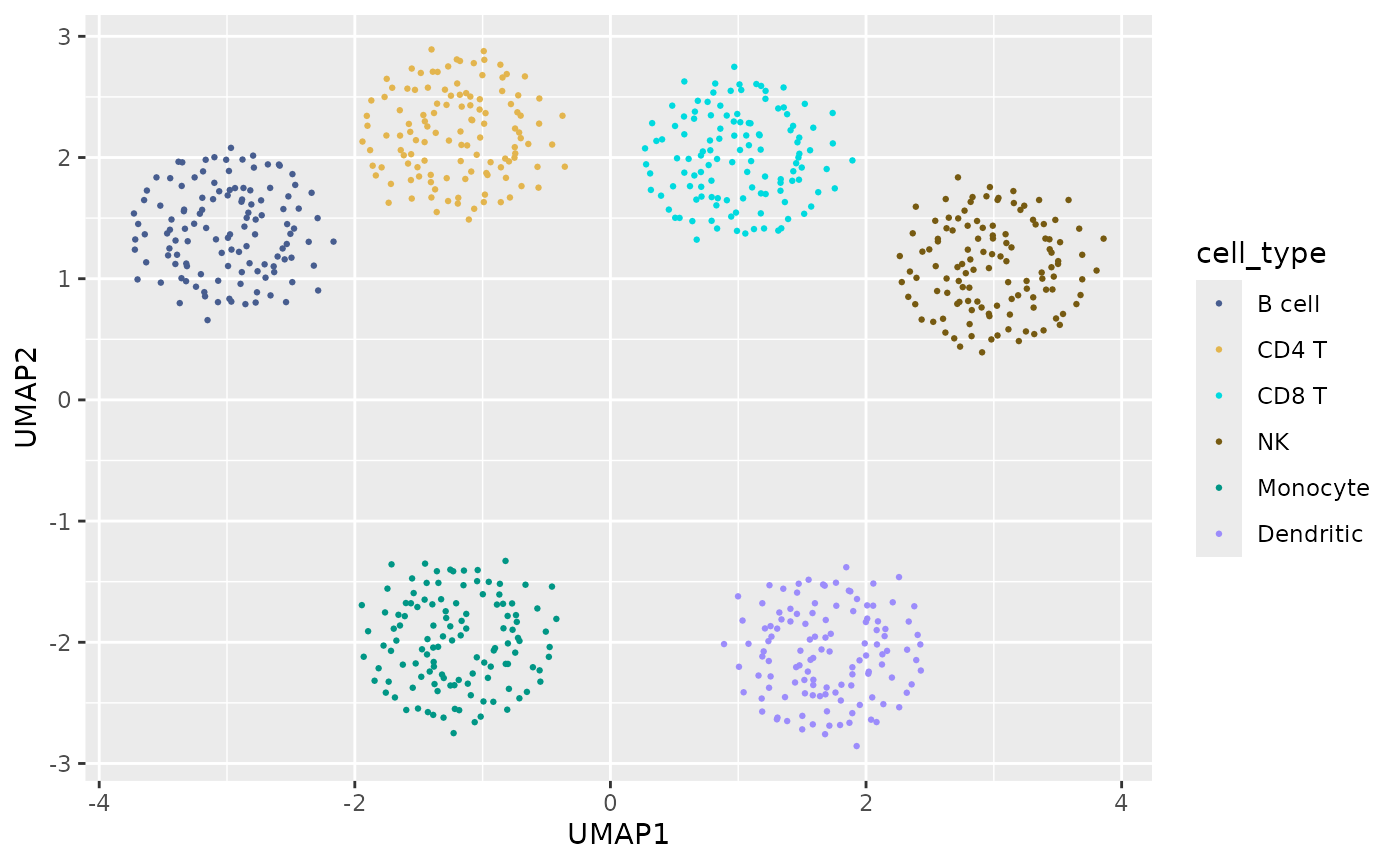
The same map is reused after filtering, so the three retained identities keep their original colors.
stimulated <- subset(
  sc_example,
  condition == "Stimulated" & cell_type %in% c("CD4 T", "NK", "Monocyte")
)

ggplot(stimulated, aes(UMAP1, UMAP2, color = cell_type)) +
  geom_point(size = 0.7) +
  scale_color_sc_map(cell_map)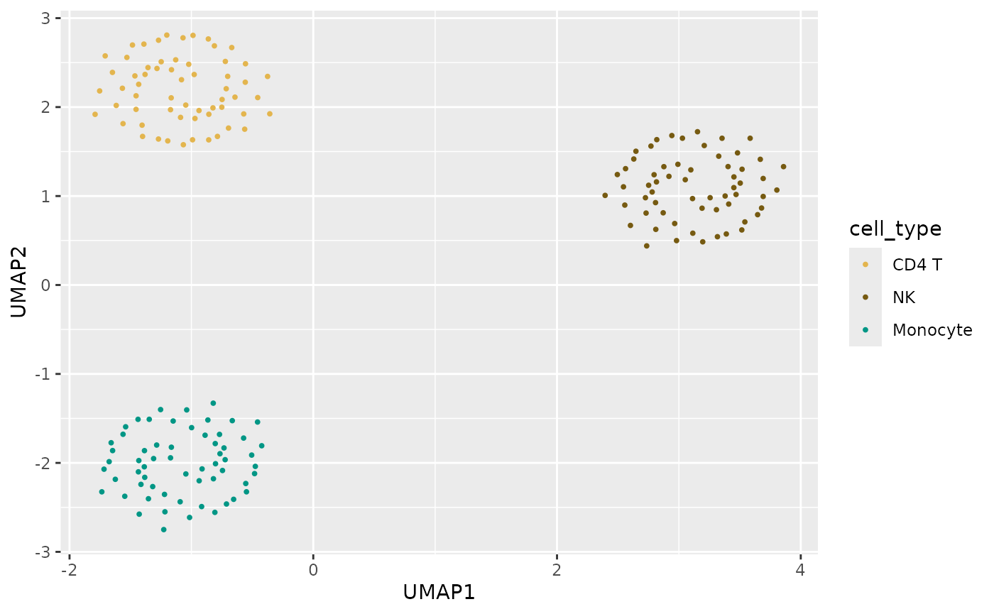
Choosing a ggplot2 scale
Choose a scale from both the mapped data and the ggplot2 aesthetic:
| Mapped data and assignment strategy |
color or colour
aesthetic |
fill aesthetic |
|---|---|---|
| Categorical, assigned for one plot | scale_color_sc_d() |
scale_fill_sc_d() |
Categorical, locked in an
sc_color_map
|
scale_color_sc_map() |
scale_fill_sc_map() |
| Numeric, shown as a gradient | scale_color_sc_c() |
scale_fill_sc_c() |
The color aesthetic controls points, lines, text, and
geometry outlines; fill controls the interiors of violins,
bars, tiles, polygons, and other filled geometries. The
scale_colour_*() functions are exact aliases of the
corresponding scale_color_*() functions. Match the scale to
the aesthetic in aes(): mapping fill = sample
requires a scale_fill_*() scale, while mapping
color = sample requires a scale_color_*()
scale.
Use the _sc_map() family when categories must keep the
same colors across figures, subsets, or reordered factors. A single map
can drive either aesthetic.
sample_map <- sc_color_map(sc_example$sample, palette = "chromatic")

ggplot(sc_example, aes(UMAP1, UMAP2, color = sample)) +
  geom_point(size = 0.5) +
  scale_color_sc_map(sample_map)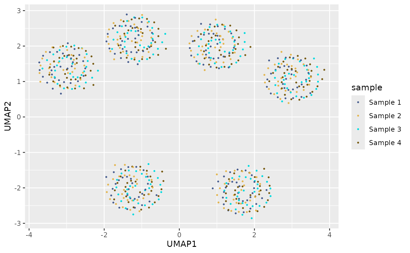
ggplot(sc_example, aes(sample, n_counts, fill = sample)) +
  geom_violin() +
  scale_y_log10() +
  scale_fill_sc_map(sample_map) +
  labs(x = NULL, y = "Library size")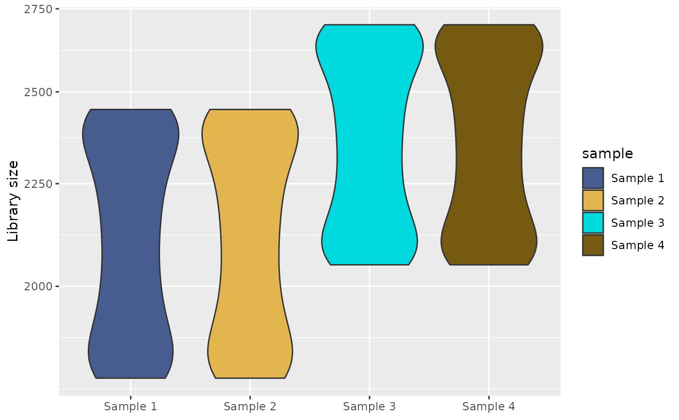
Use _sc_d() for a one-off categorical plot where a
persistent assignment is not needed. Its assignments are computed from
the discrete levels supplied to that plot.
ggplot(sc_example, aes(UMAP1, UMAP2, color = condition)) +
  geom_point(size = 0.5) +
  scale_color_sc_d("chromatic")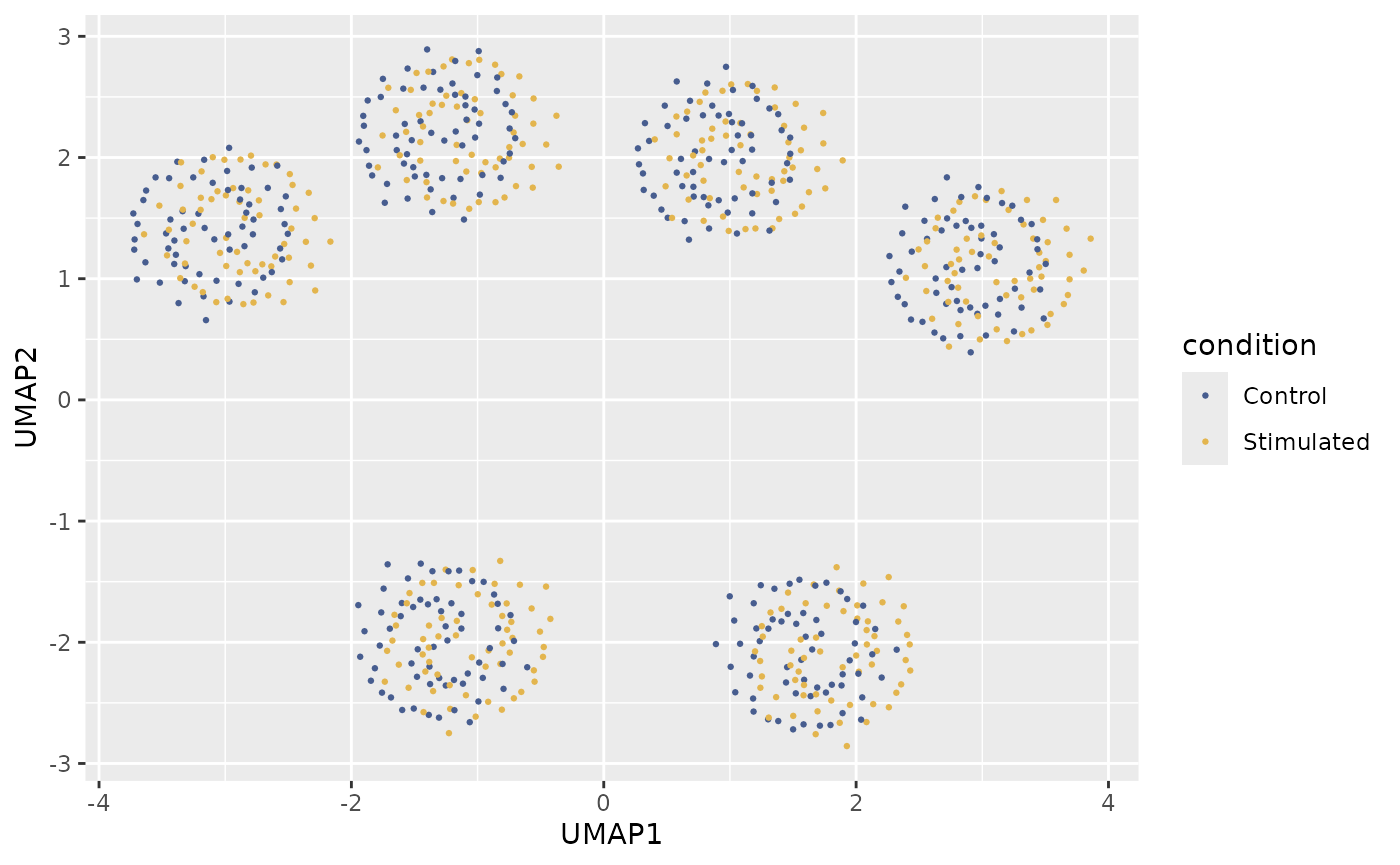
Use _sc_c() only for numeric values. Sequential,
diverging, or cyclic palettes are valid for continuous scales;
qualitative palettes are not. If a category is stored as numbers,
convert it to a factor before using _sc_d() or constructing
an sc_color_map.
These rules do not depend on the source object. For a Seurat object,
object[[]] supplies its metadata data frame and
object$sample supplies the sample vector used to construct
a map. A plot returned by another package, including pixelatorR, must
still use the scale matching the aesthetic mapped by that plot. If both
color and fill are mapped, add one scale for
each aesthetic; otherwise, use only the scale that matches
aes().
Continuous expression
ggplot(sc_example, aes(UMAP1, UMAP2, color = MS4A1)) +
  geom_point(size = 0.5) +
  scale_color_sc_c("viridis")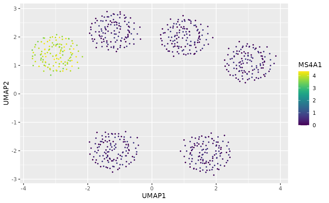
Signed scores centered at zero
midpoint = 0 changes data rescaling, not merely the
middle displayed color.
ggplot(sc_example, aes(UMAP1, UMAP2, color = signed_score)) +
  geom_point(size = 0.5) +
  scale_color_sc_c("chromatic_balance", midpoint = 0)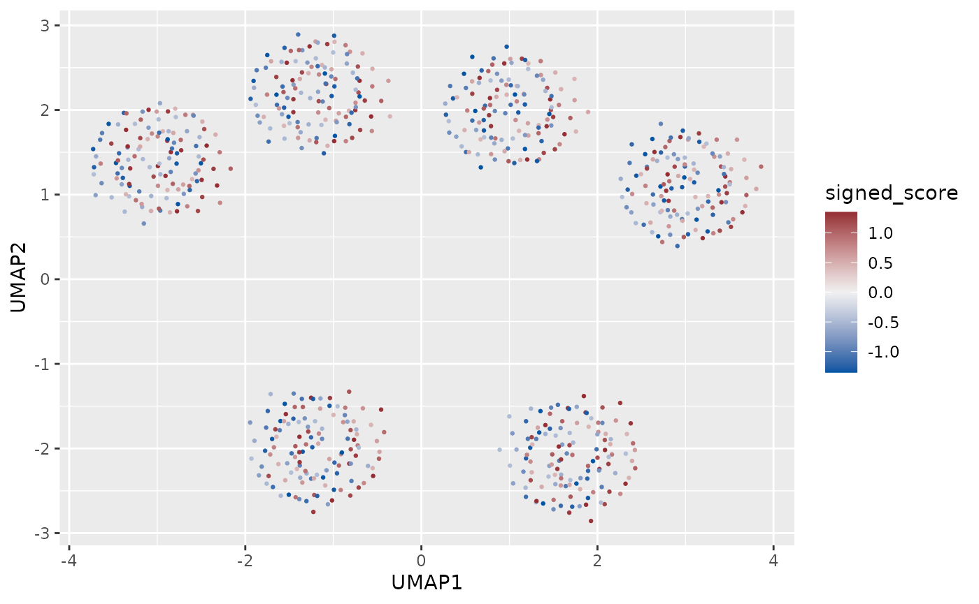
Parent lineage and child subtype colors
lineage_map <- sc_hierarchy_map(sc_example$lineage, sc_example$cell_type)

ggplot(sc_example, aes(UMAP1, UMAP2, color = cell_type)) +
  geom_point(size = 0.5) +
  scale_color_sc_map(lineage_map)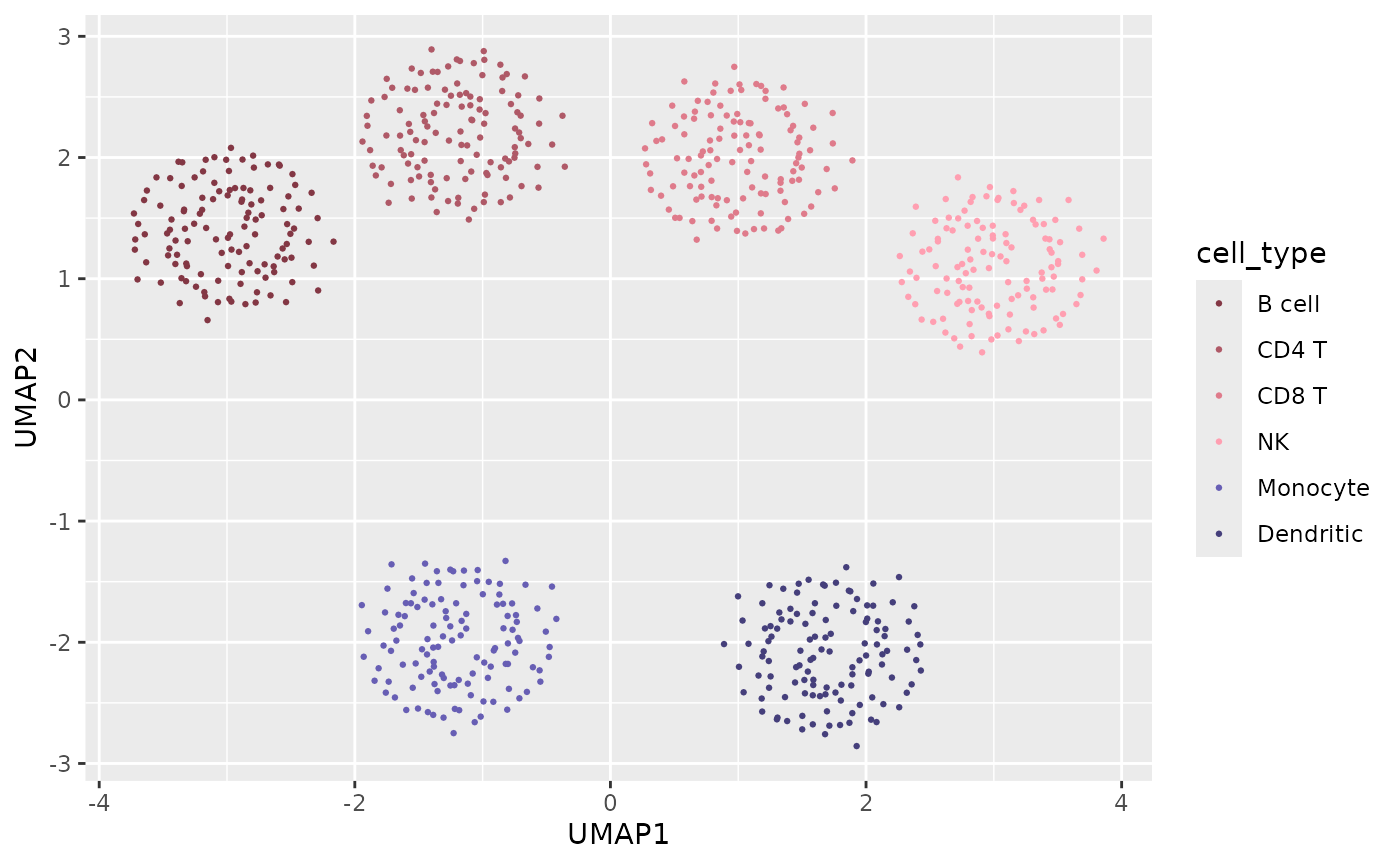
Pseudotime and QC
ggplot(sc_example, aes(UMAP1, UMAP2, color = pseudotime)) +
  geom_point(size = 0.5) +
  scale_color_sc_c("cividis")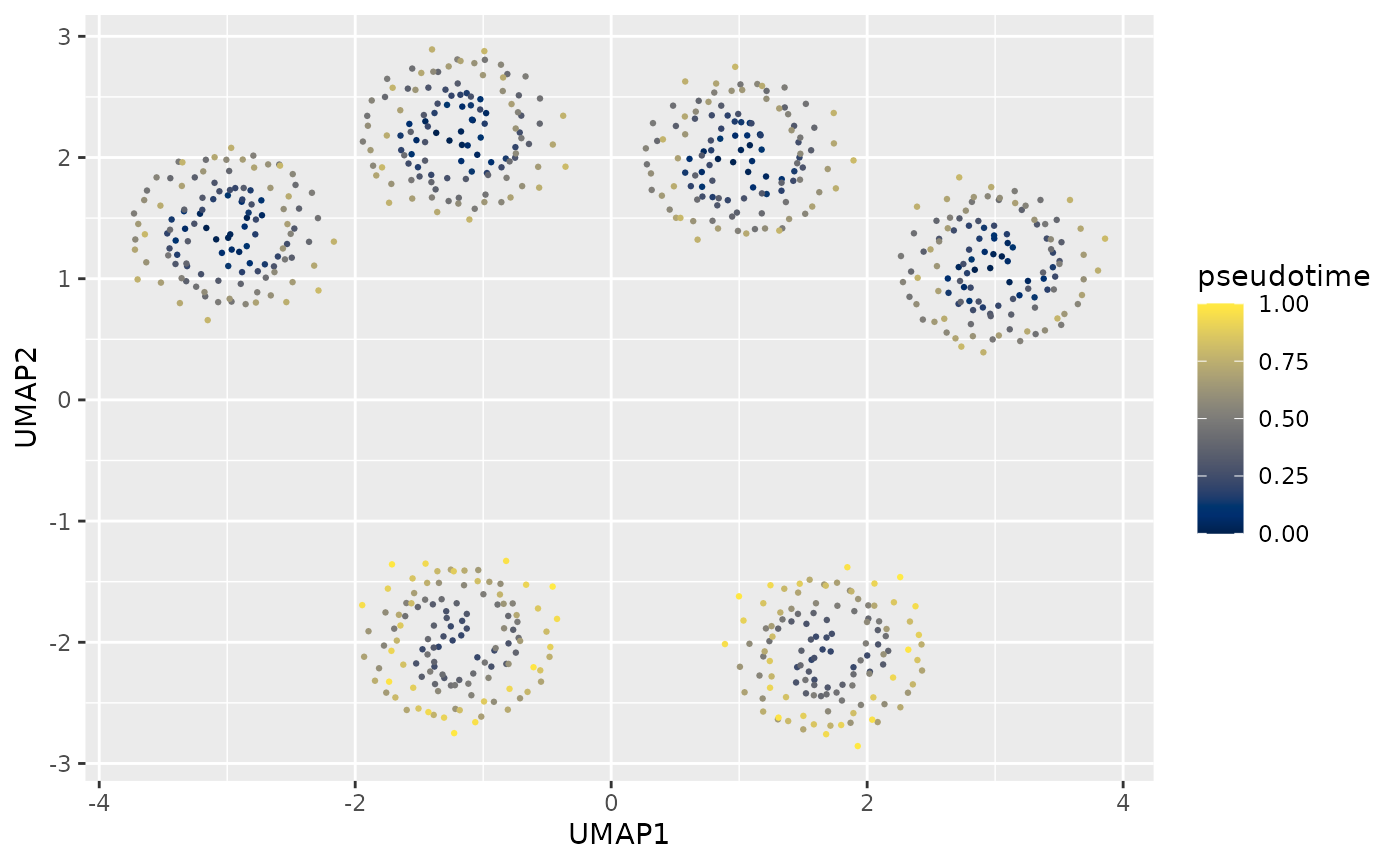
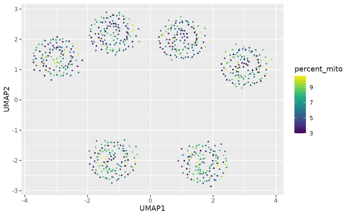
ggplot(sc_example, aes(UMAP1, UMAP2, color = percent_mito)) +
  geom_point(size = 0.5) +
  scale_color_sc_c("viridis")