14 PCA

PCA reduces the dimensionality of a multivariate data to two or three principal components, that can be visualized graphically, with minimal loss of information.

PCA is veru useful whne the varianle with the data set are highly correlated. Correlation indicates that there is redundancy in the data. Due to this redundancy, PCA can be used to reduce the original variable into smaller number of new variabeles, nameing principal components.

14.1 Read data

iris_tab <- read.csv("https://gist.githubusercontent.com/curran/a08a1080b88344b0c8a7/raw/d546eaee765268bf2f487608c537c05e22e4b221/iris.csv")

14.2 Head data

head(iris_tab)

##   sepal_length sepal_width petal_length petal_width species
## 1          5.1         3.5          1.4         0.2  setosa
## 2          4.9         3.0          1.4         0.2  setosa
## 3          4.7         3.2          1.3         0.2  setosa
## 4          4.6         3.1          1.5         0.2  setosa
## 5          5.0         3.6          1.4         0.2  setosa
## 6          5.4         3.9          1.7         0.4  setosa

14.3 Summary of the data

summary(iris_tab)

##   sepal_length    sepal_width     petal_length    petal_width   
##  Min.   :4.300   Min.   :2.000   Min.   :1.000   Min.   :0.100  
##  1st Qu.:5.100   1st Qu.:2.800   1st Qu.:1.600   1st Qu.:0.300  
##  Median :5.800   Median :3.000   Median :4.350   Median :1.300  
##  Mean   :5.843   Mean   :3.054   Mean   :3.759   Mean   :1.199  
##  3rd Qu.:6.400   3rd Qu.:3.300   3rd Qu.:5.100   3rd Qu.:1.800  
##  Max.   :7.900   Max.   :4.400   Max.   :6.900   Max.   :2.500  
##        species  
##  setosa    :50  
##  versicolor:50  
##  virginica :50  
##                 
##                 
##

14.4 Check the distribution of the data

hist(iris_tab$sepal_length)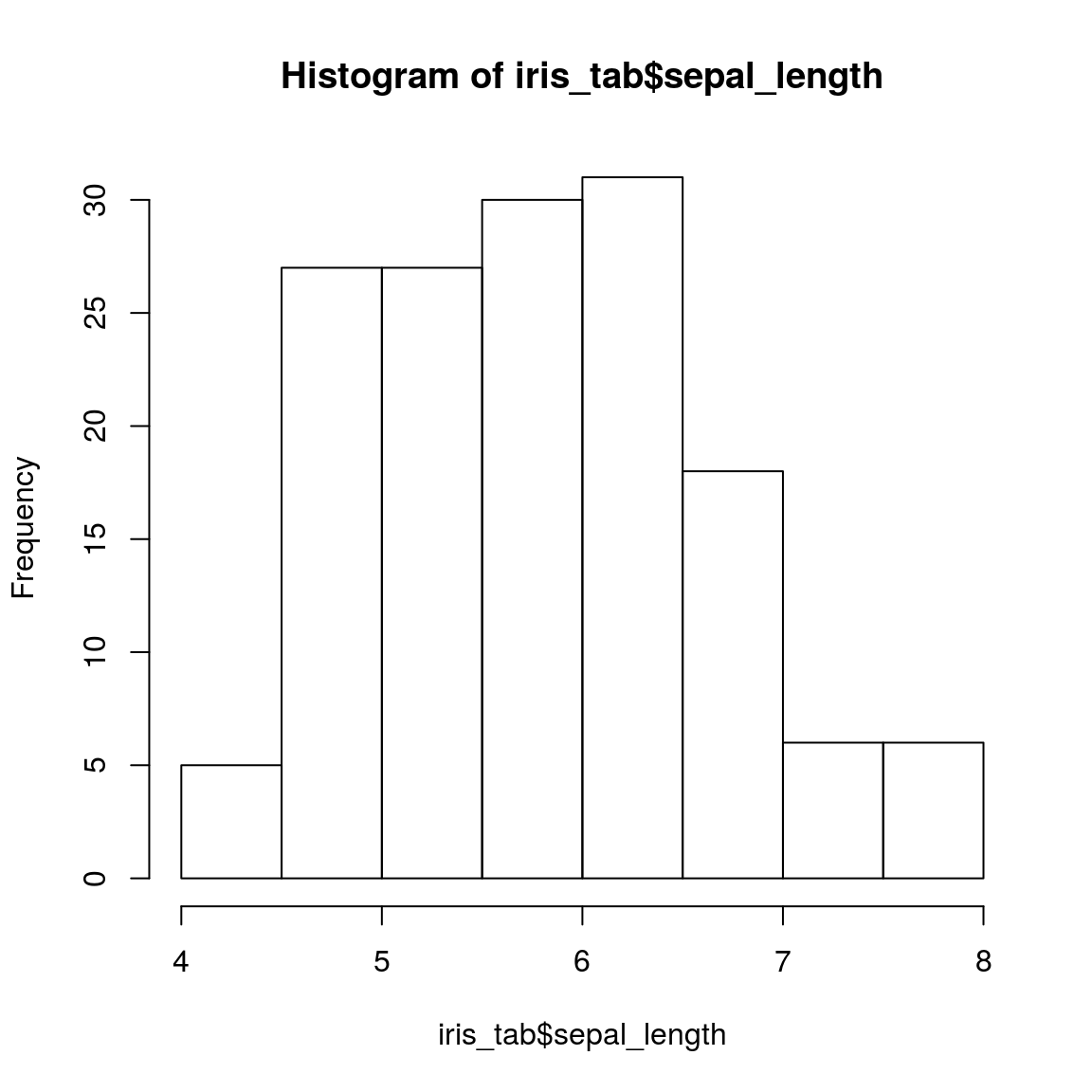

14.5 Eigendecomposition - Computing Eigenvectors and Eigenvalues

In linear algebra, an eigenvector is a non-zero vector that changes by only a scalar factor when that linear transformation is applied to it.

The eigenvectors and eigenvalues of a covariance (or correlation) matrix represent the “core” of a PCA: The eigenvectors (principal components) determine the directions of the new feature space, and the eigenvalues determine their magnitude. In other words, the eigenvalues explain the variance of the data along the new feature axes.

14.5.1 Covariance Matrix

The classic approach to PCA is to perform the eigendecomposition on the covariance matrix \(\Sigma\), which is a \(d \times d\) matrix where each element represents the covariance between two features. The covariance between two features is calculated as follows:

\(\sigma_{jk} = \frac{1}{n-1}\sum_{i=1}^{N}\left( x_{ij}-\bar{x}_j \right) \left( x_{ik}-\bar{x}_k \right).\)

We can summarize the calculation of the covariance matrix via the following matrix equation:

\(\Sigma = \frac{1}{n-1} \left( (\mathbf{X} - \mathbf{\bar{x}})^T\;(\mathbf{X} - \mathbf{\bar{x}}) \right)\)
where \(\mathbf{\bar{x}}\) is the mean vector \(\mathbf{\bar{x}} = \sum\limits_{i=1}^n x_{i}.\)

The mean vector is a \(d\)-dimensional vector where each value in this vector represents the sample mean of a feature column in the dataset.

cov_mat<-cor(iris_tab[,1:4])
cov_mat

##              sepal_length sepal_width petal_length petal_width
## sepal_length    1.0000000  -0.1093692    0.8717542   0.8179536
## sepal_width    -0.1093692   1.0000000   -0.4205161  -0.3565441
## petal_length    0.8717542  -0.4205161    1.0000000   0.9627571
## petal_width     0.8179536  -0.3565441    0.9627571   1.0000000

#install.packages("corrplot")
library(corrplot)
corrplot(cov_mat)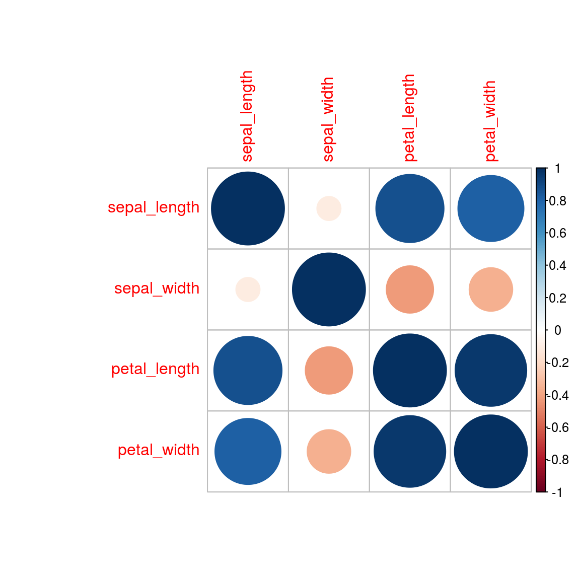

14.6 PCA with two variables

new_data = as.data.frame(cbind(petal_length = iris_tab$petal_length, petal_width = iris_tab$petal_width))
head(new_data)

##   petal_length petal_width
## 1          1.4         0.2
## 2          1.4         0.2
## 3          1.3         0.2
## 4          1.5         0.2
## 5          1.4         0.2
## 6          1.7         0.4

plot(new_data$petal_length, new_data$petal_width)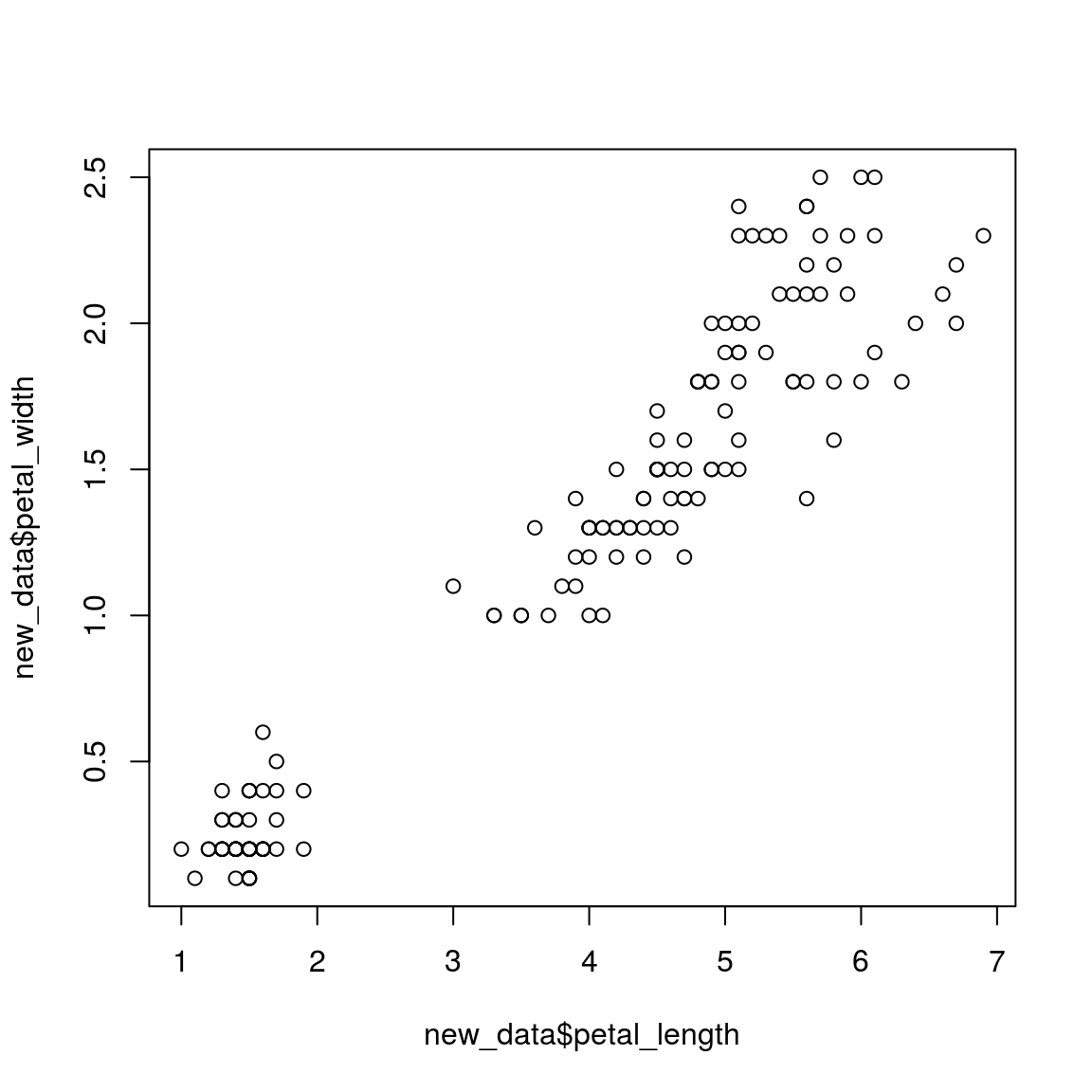

#install.packages("FactoMineR")
library("FactoMineR")
pc_2var_res = PCA(new_data)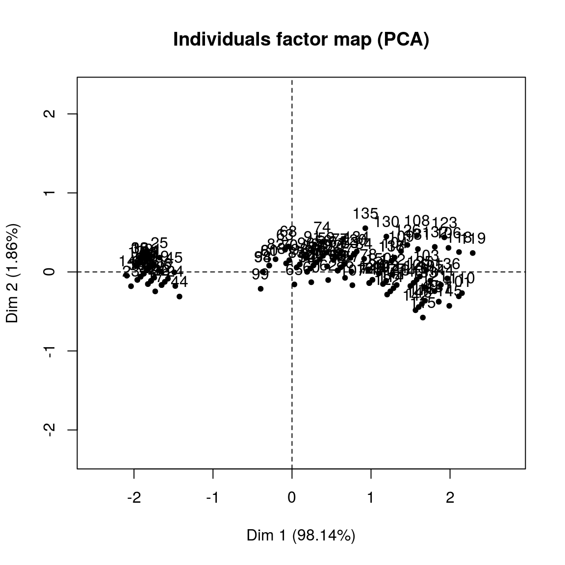

print(pc_2var_res)

## **Results for the Principal Component Analysis (PCA)**
## The analysis was performed on 150 individuals, described by 2 variables
## *The results are available in the following objects:
## 
##    name               description                          
## 1  "$eig"             "eigenvalues"                        
## 2  "$var"             "results for the variables"          
## 3  "$var$coord"       "coord. for the variables"           
## 4  "$var$cor"         "correlations variables - dimensions"
## 5  "$var$cos2"        "cos2 for the variables"             
## 6  "$var$contrib"     "contributions of the variables"     
## 7  "$ind"             "results for the individuals"        
## 8  "$ind$coord"       "coord. for the individuals"         
## 9  "$ind$cos2"        "cos2 for the individuals"           
## 10 "$ind$contrib"     "contributions of the individuals"   
## 11 "$call"            "summary statistics"                 
## 12 "$call$centre"     "mean of the variables"              
## 13 "$call$ecart.type" "standard error of the variables"    
## 14 "$call$row.w"      "weights for the individuals"        
## 15 "$call$col.w"      "weights for the variables"

#install.packages("FactoInvestigate")
#library(FactoInvestigate)
#Investigate(pc_2var_res, document = "pdf_document")

Next, we perform an eigendecomposition on the covariance matrix:

eigen(cov_mat)

## eigen() decomposition
## $values
## [1] 2.91081808 0.92122093 0.14735328 0.02060771
## 
## $vectors
##            [,1]        [,2]       [,3]       [,4]
## [1,]  0.5223716 -0.37231836  0.7210168  0.2619956
## [2,] -0.2633549 -0.92555649 -0.2420329 -0.1241348
## [3,]  0.5812540 -0.02109478 -0.1408923 -0.8011543
## [4,]  0.5656110 -0.06541577 -0.6338014  0.5235463

14.7 PCA on `wine` data

14.7.1 Read the `wine` data

wine <- read.csv("data/wine.csv", header=T)
knitr::kable(wine)

Wine	Alcohol	Malic.acid	Ash	Acl	Mg	Phenols	Flavanoids	Nonflavanoid.phenols	Proanth	Color.int	Hue	OD	Proline
1	14.23	1.71	2.43	15.6	127	2.80	3.06	0.28	2.29	5.640000	1.040	3.92	1065
1	13.20	1.78	2.14	11.2	100	2.65	2.76	0.26	1.28	4.380000	1.050	3.40	1050
1	13.16	2.36	2.67	18.6	101	2.80	3.24	0.30	2.81	5.680000	1.030	3.17	1185
1	14.37	1.95	2.50	16.8	113	3.85	3.49	0.24	2.18	7.800000	0.860	3.45	1480
1	13.24	2.59	2.87	21.0	118	2.80	2.69	0.39	1.82	4.320000	1.040	2.93	735
1	14.20	1.76	2.45	15.2	112	3.27	3.39	0.34	1.97	6.750000	1.050	2.85	1450
1	14.39	1.87	2.45	14.6	96	2.50	2.52	0.30	1.98	5.250000	1.020	3.58	1290
1	14.06	2.15	2.61	17.6	121	2.60	2.51	0.31	1.25	5.050000	1.060	3.58	1295
1	14.83	1.64	2.17	14.0	97	2.80	2.98	0.29	1.98	5.200000	1.080	2.85	1045
1	13.86	1.35	2.27	16.0	98	2.98	3.15	0.22	1.85	7.220000	1.010	3.55	1045
1	14.10	2.16	2.30	18.0	105	2.95	3.32	0.22	2.38	5.750000	1.250	3.17	1510
1	14.12	1.48	2.32	16.8	95	2.20	2.43	0.26	1.57	5.000000	1.170	2.82	1280
1	13.75	1.73	2.41	16.0	89	2.60	2.76	0.29	1.81	5.600000	1.150	2.90	1320
1	14.75	1.73	2.39	11.4	91	3.10	3.69	0.43	2.81	5.400000	1.250	2.73	1150
1	14.38	1.87	2.38	12.0	102	3.30	3.64	0.29	2.96	7.500000	1.200	3.00	1547
1	13.63	1.81	2.70	17.2	112	2.85	2.91	0.30	1.46	7.300000	1.280	2.88	1310
1	14.30	1.92	2.72	20.0	120	2.80	3.14	0.33	1.97	6.200000	1.070	2.65	1280
1	13.83	1.57	2.62	20.0	115	2.95	3.40	0.40	1.72	6.600000	1.130	2.57	1130
1	14.19	1.59	2.48	16.5	108	3.30	3.93	0.32	1.86	8.700000	1.230	2.82	1680
1	13.64	3.10	2.56	15.2	116	2.70	3.03	0.17	1.66	5.100000	0.960	3.36	845
1	14.06	1.63	2.28	16.0	126	3.00	3.17	0.24	2.10	5.650000	1.090	3.71	780
1	12.93	3.80	2.65	18.6	102	2.41	2.41	0.25	1.98	4.500000	1.030	3.52	770
1	13.71	1.86	2.36	16.6	101	2.61	2.88	0.27	1.69	3.800000	1.110	4.00	1035
1	12.85	1.60	2.52	17.8	95	2.48	2.37	0.26	1.46	3.930000	1.090	3.63	1015
1	13.50	1.81	2.61	20.0	96	2.53	2.61	0.28	1.66	3.520000	1.120	3.82	845
1	13.05	2.05	3.22	25.0	124	2.63	2.68	0.47	1.92	3.580000	1.130	3.20	830
1	13.39	1.77	2.62	16.1	93	2.85	2.94	0.34	1.45	4.800000	0.920	3.22	1195
1	13.30	1.72	2.14	17.0	94	2.40	2.19	0.27	1.35	3.950000	1.020	2.77	1285
1	13.87	1.90	2.80	19.4	107	2.95	2.97	0.37	1.76	4.500000	1.250	3.40	915
1	14.02	1.68	2.21	16.0	96	2.65	2.33	0.26	1.98	4.700000	1.040	3.59	1035
1	13.73	1.50	2.70	22.5	101	3.00	3.25	0.29	2.38	5.700000	1.190	2.71	1285
1	13.58	1.66	2.36	19.1	106	2.86	3.19	0.22	1.95	6.900000	1.090	2.88	1515
1	13.68	1.83	2.36	17.2	104	2.42	2.69	0.42	1.97	3.840000	1.230	2.87	990
1	13.76	1.53	2.70	19.5	132	2.95	2.74	0.50	1.35	5.400000	1.250	3.00	1235
1	13.51	1.80	2.65	19.0	110	2.35	2.53	0.29	1.54	4.200000	1.100	2.87	1095
1	13.48	1.81	2.41	20.5	100	2.70	2.98	0.26	1.86	5.100000	1.040	3.47	920
1	13.28	1.64	2.84	15.5	110	2.60	2.68	0.34	1.36	4.600000	1.090	2.78	880
1	13.05	1.65	2.55	18.0	98	2.45	2.43	0.29	1.44	4.250000	1.120	2.51	1105
1	13.07	1.50	2.10	15.5	98	2.40	2.64	0.28	1.37	3.700000	1.180	2.69	1020
1	14.22	3.99	2.51	13.2	128	3.00	3.04	0.20	2.08	5.100000	0.890	3.53	760
1	13.56	1.71	2.31	16.2	117	3.15	3.29	0.34	2.34	6.130000	0.950	3.38	795
1	13.41	3.84	2.12	18.8	90	2.45	2.68	0.27	1.48	4.280000	0.910	3.00	1035
1	13.88	1.89	2.59	15.0	101	3.25	3.56	0.17	1.70	5.430000	0.880	3.56	1095
1	13.24	3.98	2.29	17.5	103	2.64	2.63	0.32	1.66	4.360000	0.820	3.00	680
1	13.05	1.77	2.10	17.0	107	3.00	3.00	0.28	2.03	5.040000	0.880	3.35	885
1	14.21	4.04	2.44	18.9	111	2.85	2.65	0.30	1.25	5.240000	0.870	3.33	1080
1	14.38	3.59	2.28	16.0	102	3.25	3.17	0.27	2.19	4.900000	1.040	3.44	1065
1	13.90	1.68	2.12	16.0	101	3.10	3.39	0.21	2.14	6.100000	0.910	3.33	985
1	14.10	2.02	2.40	18.8	103	2.75	2.92	0.32	2.38	6.200000	1.070	2.75	1060
1	13.94	1.73	2.27	17.4	108	2.88	3.54	0.32	2.08	8.900000	1.120	3.10	1260
1	13.05	1.73	2.04	12.4	92	2.72	3.27	0.17	2.91	7.200000	1.120	2.91	1150
1	13.83	1.65	2.60	17.2	94	2.45	2.99	0.22	2.29	5.600000	1.240	3.37	1265
1	13.82	1.75	2.42	14.0	111	3.88	3.74	0.32	1.87	7.050000	1.010	3.26	1190
1	13.77	1.90	2.68	17.1	115	3.00	2.79	0.39	1.68	6.300000	1.130	2.93	1375
1	13.74	1.67	2.25	16.4	118	2.60	2.90	0.21	1.62	5.850000	0.920	3.20	1060
1	13.56	1.73	2.46	20.5	116	2.96	2.78	0.20	2.45	6.250000	0.980	3.03	1120
1	14.22	1.70	2.30	16.3	118	3.20	3.00	0.26	2.03	6.380000	0.940	3.31	970
1	13.29	1.97	2.68	16.8	102	3.00	3.23	0.31	1.66	6.000000	1.070	2.84	1270
1	13.72	1.43	2.50	16.7	108	3.40	3.67	0.19	2.04	6.800000	0.890	2.87	1285
2	12.37	0.94	1.36	10.6	88	1.98	0.57	0.28	0.42	1.950000	1.050	1.82	520
2	12.33	1.10	2.28	16.0	101	2.05	1.09	0.63	0.41	3.270000	1.250	1.67	680
2	12.64	1.36	2.02	16.8	100	2.02	1.41	0.53	0.62	5.750000	0.980	1.59	450
2	13.67	1.25	1.92	18.0	94	2.10	1.79	0.32	0.73	3.800000	1.230	2.46	630
2	12.37	1.13	2.16	19.0	87	3.50	3.10	0.19	1.87	4.450000	1.220	2.87	420
2	12.17	1.45	2.53	19.0	104	1.89	1.75	0.45	1.03	2.950000	1.450	2.23	355
2	12.37	1.21	2.56	18.1	98	2.42	2.65	0.37	2.08	4.600000	1.190	2.30	678
2	13.11	1.01	1.70	15.0	78	2.98	3.18	0.26	2.28	5.300000	1.120	3.18	502
2	12.37	1.17	1.92	19.6	78	2.11	2.00	0.27	1.04	4.680000	1.120	3.48	510
2	13.34	0.94	2.36	17.0	110	2.53	1.30	0.55	0.42	3.170000	1.020	1.93	750
2	12.21	1.19	1.75	16.8	151	1.85	1.28	0.14	2.50	2.850000	1.280	3.07	718
2	12.29	1.61	2.21	20.4	103	1.10	1.02	0.37	1.46	3.050000	0.906	1.82	870
2	13.86	1.51	2.67	25.0	86	2.95	2.86	0.21	1.87	3.380000	1.360	3.16	410
2	13.49	1.66	2.24	24.0	87	1.88	1.84	0.27	1.03	3.740000	0.980	2.78	472
2	12.99	1.67	2.60	30.0	139	3.30	2.89	0.21	1.96	3.350000	1.310	3.50	985
2	11.96	1.09	2.30	21.0	101	3.38	2.14	0.13	1.65	3.210000	0.990	3.13	886
2	11.66	1.88	1.92	16.0	97	1.61	1.57	0.34	1.15	3.800000	1.230	2.14	428
2	13.03	0.90	1.71	16.0	86	1.95	2.03	0.24	1.46	4.600000	1.190	2.48	392
2	11.84	2.89	2.23	18.0	112	1.72	1.32	0.43	0.95	2.650000	0.960	2.52	500
2	12.33	0.99	1.95	14.8	136	1.90	1.85	0.35	2.76	3.400000	1.060	2.31	750
2	12.70	3.87	2.40	23.0	101	2.83	2.55	0.43	1.95	2.570000	1.190	3.13	463
2	12.00	0.92	2.00	19.0	86	2.42	2.26	0.30	1.43	2.500000	1.380	3.12	278
2	12.72	1.81	2.20	18.8	86	2.20	2.53	0.26	1.77	3.900000	1.160	3.14	714
2	12.08	1.13	2.51	24.0	78	2.00	1.58	0.40	1.40	2.200000	1.310	2.72	630
2	13.05	3.86	2.32	22.5	85	1.65	1.59	0.61	1.62	4.800000	0.840	2.01	515
2	11.84	0.89	2.58	18.0	94	2.20	2.21	0.22	2.35	3.050000	0.790	3.08	520
2	12.67	0.98	2.24	18.0	99	2.20	1.94	0.30	1.46	2.620000	1.230	3.16	450
2	12.16	1.61	2.31	22.8	90	1.78	1.69	0.43	1.56	2.450000	1.330	2.26	495
2	11.65	1.67	2.62	26.0	88	1.92	1.61	0.40	1.34	2.600000	1.360	3.21	562
2	11.64	2.06	2.46	21.6	84	1.95	1.69	0.48	1.35	2.800000	1.000	2.75	680
2	12.08	1.33	2.30	23.6	70	2.20	1.59	0.42	1.38	1.740000	1.070	3.21	625
2	12.08	1.83	2.32	18.5	81	1.60	1.50	0.52	1.64	2.400000	1.080	2.27	480
2	12.00	1.51	2.42	22.0	86	1.45	1.25	0.50	1.63	3.600000	1.050	2.65	450
2	12.69	1.53	2.26	20.7	80	1.38	1.46	0.58	1.62	3.050000	0.960	2.06	495
2	12.29	2.83	2.22	18.0	88	2.45	2.25	0.25	1.99	2.150000	1.150	3.30	290
2	11.62	1.99	2.28	18.0	98	3.02	2.26	0.17	1.35	3.250000	1.160	2.96	345
2	12.47	1.52	2.20	19.0	162	2.50	2.27	0.32	3.28	2.600000	1.160	2.63	937
2	11.81	2.12	2.74	21.5	134	1.60	0.99	0.14	1.56	2.500000	0.950	2.26	625
2	12.29	1.41	1.98	16.0	85	2.55	2.50	0.29	1.77	2.900000	1.230	2.74	428
2	12.37	1.07	2.10	18.5	88	3.52	3.75	0.24	1.95	4.500000	1.040	2.77	660
2	12.29	3.17	2.21	18.0	88	2.85	2.99	0.45	2.81	2.300000	1.420	2.83	406
2	12.08	2.08	1.70	17.5	97	2.23	2.17	0.26	1.40	3.300000	1.270	2.96	710
2	12.60	1.34	1.90	18.5	88	1.45	1.36	0.29	1.35	2.450000	1.040	2.77	562
2	12.34	2.45	2.46	21.0	98	2.56	2.11	0.34	1.31	2.800000	0.800	3.38	438
2	11.82	1.72	1.88	19.5	86	2.50	1.64	0.37	1.42	2.060000	0.940	2.44	415
2	12.51	1.73	1.98	20.5	85	2.20	1.92	0.32	1.48	2.940000	1.040	3.57	672
2	12.42	2.55	2.27	22.0	90	1.68	1.84	0.66	1.42	2.700000	0.860	3.30	315
2	12.25	1.73	2.12	19.0	80	1.65	2.03	0.37	1.63	3.400000	1.000	3.17	510
2	12.72	1.75	2.28	22.5	84	1.38	1.76	0.48	1.63	3.300000	0.880	2.42	488
2	12.22	1.29	1.94	19.0	92	2.36	2.04	0.39	2.08	2.700000	0.860	3.02	312
2	11.61	1.35	2.70	20.0	94	2.74	2.92	0.29	2.49	2.650000	0.960	3.26	680
2	11.46	3.74	1.82	19.5	107	3.18	2.58	0.24	3.58	2.900000	0.750	2.81	562
2	12.52	2.43	2.17	21.0	88	2.55	2.27	0.26	1.22	2.000000	0.900	2.78	325
2	11.76	2.68	2.92	20.0	103	1.75	2.03	0.60	1.05	3.800000	1.230	2.50	607
2	11.41	0.74	2.50	21.0	88	2.48	2.01	0.42	1.44	3.080000	1.100	2.31	434
2	12.08	1.39	2.50	22.5	84	2.56	2.29	0.43	1.04	2.900000	0.930	3.19	385
2	11.03	1.51	2.20	21.5	85	2.46	2.17	0.52	2.01	1.900000	1.710	2.87	407
2	11.82	1.47	1.99	20.8	86	1.98	1.60	0.30	1.53	1.950000	0.950	3.33	495
2	12.42	1.61	2.19	22.5	108	2.00	2.09	0.34	1.61	2.060000	1.060	2.96	345
2	12.77	3.43	1.98	16.0	80	1.63	1.25	0.43	0.83	3.400000	0.700	2.12	372
2	12.00	3.43	2.00	19.0	87	2.00	1.64	0.37	1.87	1.280000	0.930	3.05	564
2	11.45	2.40	2.42	20.0	96	2.90	2.79	0.32	1.83	3.250000	0.800	3.39	625
2	11.56	2.05	3.23	28.5	119	3.18	5.08	0.47	1.87	6.000000	0.930	3.69	465
2	12.42	4.43	2.73	26.5	102	2.20	2.13	0.43	1.71	2.080000	0.920	3.12	365
2	13.05	5.80	2.13	21.5	86	2.62	2.65	0.30	2.01	2.600000	0.730	3.10	380
2	11.87	4.31	2.39	21.0	82	2.86	3.03	0.21	2.91	2.800000	0.750	3.64	380
2	12.07	2.16	2.17	21.0	85	2.60	2.65	0.37	1.35	2.760000	0.860	3.28	378
2	12.43	1.53	2.29	21.5	86	2.74	3.15	0.39	1.77	3.940000	0.690	2.84	352
2	11.79	2.13	2.78	28.5	92	2.13	2.24	0.58	1.76	3.000000	0.970	2.44	466
2	12.37	1.63	2.30	24.5	88	2.22	2.45	0.40	1.90	2.120000	0.890	2.78	342
2	12.04	4.30	2.38	22.0	80	2.10	1.75	0.42	1.35	2.600000	0.790	2.57	580
3	12.86	1.35	2.32	18.0	122	1.51	1.25	0.21	0.94	4.100000	0.760	1.29	630
3	12.88	2.99	2.40	20.0	104	1.30	1.22	0.24	0.83	5.400000	0.740	1.42	530
3	12.81	2.31	2.40	24.0	98	1.15	1.09	0.27	0.83	5.700000	0.660	1.36	560
3	12.70	3.55	2.36	21.5	106	1.70	1.20	0.17	0.84	5.000000	0.780	1.29	600
3	12.51	1.24	2.25	17.5	85	2.00	0.58	0.60	1.25	5.450000	0.750	1.51	650
3	12.60	2.46	2.20	18.5	94	1.62	0.66	0.63	0.94	7.100000	0.730	1.58	695
3	12.25	4.72	2.54	21.0	89	1.38	0.47	0.53	0.80	3.850000	0.750	1.27	720
3	12.53	5.51	2.64	25.0	96	1.79	0.60	0.63	1.10	5.000000	0.820	1.69	515
3	13.49	3.59	2.19	19.5	88	1.62	0.48	0.58	0.88	5.700000	0.810	1.82	580
3	12.84	2.96	2.61	24.0	101	2.32	0.60	0.53	0.81	4.920000	0.890	2.15	590
3	12.93	2.81	2.70	21.0	96	1.54	0.50	0.53	0.75	4.600000	0.770	2.31	600
3	13.36	2.56	2.35	20.0	89	1.40	0.50	0.37	0.64	5.600000	0.700	2.47	780
3	13.52	3.17	2.72	23.5	97	1.55	0.52	0.50	0.55	4.350000	0.890	2.06	520
3	13.62	4.95	2.35	20.0	92	2.00	0.80	0.47	1.02	4.400000	0.910	2.05	550
3	12.25	3.88	2.20	18.5	112	1.38	0.78	0.29	1.14	8.210000	0.650	2.00	855
3	13.16	3.57	2.15	21.0	102	1.50	0.55	0.43	1.30	4.000000	0.600	1.68	830
3	13.88	5.04	2.23	20.0	80	0.98	0.34	0.40	0.68	4.900000	0.580	1.33	415
3	12.87	4.61	2.48	21.5	86	1.70	0.65	0.47	0.86	7.650000	0.540	1.86	625
3	13.32	3.24	2.38	21.5	92	1.93	0.76	0.45	1.25	8.420000	0.550	1.62	650
3	13.08	3.90	2.36	21.5	113	1.41	1.39	0.34	1.14	9.400000	0.570	1.33	550
3	13.50	3.12	2.62	24.0	123	1.40	1.57	0.22	1.25	8.600000	0.590	1.30	500
3	12.79	2.67	2.48	22.0	112	1.48	1.36	0.24	1.26	10.800000	0.480	1.47	480
3	13.11	1.90	2.75	25.5	116	2.20	1.28	0.26	1.56	7.100000	0.610	1.33	425
3	13.23	3.30	2.28	18.5	98	1.80	0.83	0.61	1.87	10.520000	0.560	1.51	675
3	12.58	1.29	2.10	20.0	103	1.48	0.58	0.53	1.40	7.600000	0.580	1.55	640
3	13.17	5.19	2.32	22.0	93	1.74	0.63	0.61	1.55	7.900000	0.600	1.48	725
3	13.84	4.12	2.38	19.5	89	1.80	0.83	0.48	1.56	9.010000	0.570	1.64	480
3	12.45	3.03	2.64	27.0	97	1.90	0.58	0.63	1.14	7.500000	0.670	1.73	880
3	14.34	1.68	2.70	25.0	98	2.80	1.31	0.53	2.70	13.000000	0.570	1.96	660
3	13.48	1.67	2.64	22.5	89	2.60	1.10	0.52	2.29	11.750000	0.570	1.78	620
3	12.36	3.83	2.38	21.0	88	2.30	0.92	0.50	1.04	7.650000	0.560	1.58	520
3	13.69	3.26	2.54	20.0	107	1.83	0.56	0.50	0.80	5.880000	0.960	1.82	680
3	12.85	3.27	2.58	22.0	106	1.65	0.60	0.60	0.96	5.580000	0.870	2.11	570
3	12.96	3.45	2.35	18.5	106	1.39	0.70	0.40	0.94	5.280000	0.680	1.75	675
3	13.78	2.76	2.30	22.0	90	1.35	0.68	0.41	1.03	9.580000	0.700	1.68	615
3	13.73	4.36	2.26	22.5	88	1.28	0.47	0.52	1.15	6.620000	0.780	1.75	520
3	13.45	3.70	2.60	23.0	111	1.70	0.92	0.43	1.46	10.680000	0.850	1.56	695
3	12.82	3.37	2.30	19.5	88	1.48	0.66	0.40	0.97	10.260000	0.720	1.75	685
3	13.58	2.58	2.69	24.5	105	1.55	0.84	0.39	1.54	8.660000	0.740	1.80	750
3	13.40	4.60	2.86	25.0	112	1.98	0.96	0.27	1.11	8.500000	0.670	1.92	630
3	12.20	3.03	2.32	19.0	96	1.25	0.49	0.40	0.73	5.500000	0.660	1.83	510
3	12.77	2.39	2.28	19.5	86	1.39	0.51	0.48	0.64	9.899999	0.570	1.63	470
3	14.16	2.51	2.48	20.0	91	1.68	0.70	0.44	1.24	9.700000	0.620	1.71	660
3	13.71	5.65	2.45	20.5	95	1.68	0.61	0.52	1.06	7.700000	0.640	1.74	740
3	13.40	3.91	2.48	23.0	102	1.80	0.75	0.43	1.41	7.300000	0.700	1.56	750
3	13.27	4.28	2.26	20.0	120	1.59	0.69	0.43	1.35	10.200000	0.590	1.56	835
3	13.17	2.59	2.37	20.0	120	1.65	0.68	0.53	1.46	9.300000	0.600	1.62	840
3	14.13	4.10	2.74	24.5	96	2.05	0.76	0.56	1.35	9.200000	0.610	1.60	560

14.7.2 Description of each column

wine_desc <- read.table("data/wine_data_desc.tsv", sep="\t", header = T)
knitr::kable(wine_desc)

colname	description
Type	The type of wine, into one of three classes, 1 (59 obs), 2(71 obs), and 3 (48 obs).
Alcohol	Alcohol
Malic	Malic acid
Ash	Ash
Alcalinity	Alcalinity of ash
Magnesium	Magnesium
Phenols	Total phenols
Flavanoids	Flavanoids
Nonflavanoids	Nonflavanoid phenols
Proanthocyanins	Proanthocyanins
Color	Color intensity.
Hue	Hue
Dilution	D280/OD315 of diluted wines.
Proline	Proline

library(corrplot)
dim(wine)

## [1] 178  14

wine_x<-wine[, 2:14]
cor_matrix<-cor(wine_x)

# method = "square", ellipse, number, shade, color, pie
# type = upper, lower, full(default)
corrplot(cor_matrix, method="circle", type = "upper")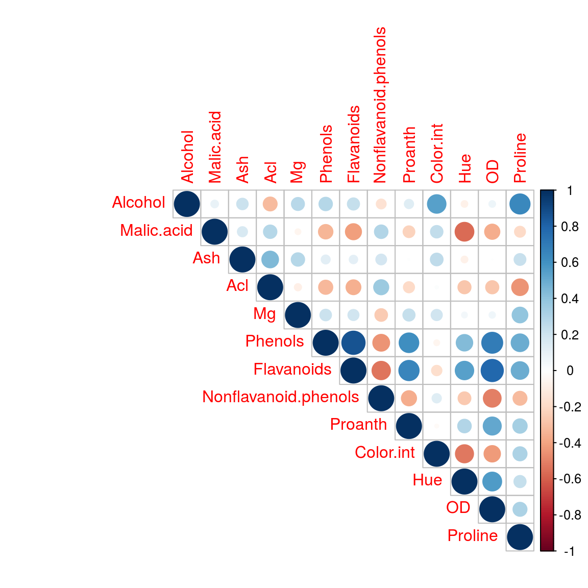

corrplot.mixed(cor_matrix)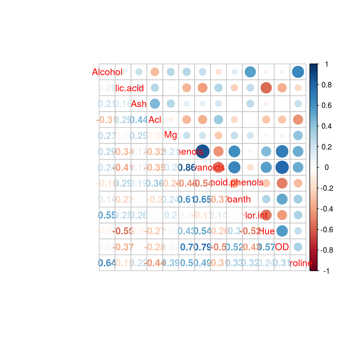

14.7.3 Example

Depends on the goal of your analysis. Some common practices, some of which are mentioned in whuber’s link:

Standardizing is usually done when the variables on which the PCA is performed are not measured on the same scale. Note that standardizing implies assigning equal importance to all variables. If they are not measured on the same scale and you choose to work on the non standardized variables, it is often the case that each PC is dominated by a single variable and you just get a sort of ordering of the variables by their variance. (One of the loadings of each (early) component will be close to +1 or -1.) The two methods often lead to different results, as you have experienced.

Intuitive example:

Suppose you have two variables: the height of a tree and the girth of the same tree. We will convert the volume to a factor: a tree will be high in volume if its volume is bigger than 20 cubic feet, and low in volume otherwise. We will use the trees dataset which comes preloaded in R

data(trees)
tree.girth<-trees[,1]
tree.height<-trees[,2]
tree.vol<-as.factor(ifelse(trees[,3]>20,"high","low"))

Now suppose that the height was actually measured in miles instead of feet.

tree.height<-tree.height/5280
tree<-cbind(tree.height,tree.girth)

#do the PCA
tree.pca<-princomp(tree)
summary(tree.pca)

## Importance of components:
##                           Comp.1       Comp.2
## Standard deviation     3.0871086 1.014551e-03
## Proportion of Variance 0.9999999 1.080050e-07
## Cumulative Proportion  0.9999999 1.000000e+00

The first component explains almost 100% of the variability in the data. The loadings:

loadings(tree.pca)

## 
## Loadings:
##             Comp.1 Comp.2
## tree.height        1     
## tree.girth  1            
## 
##                Comp.1 Comp.2
## SS loadings       1.0    1.0
## Proportion Var    0.5    0.5
## Cumulative Var    0.5    1.0

biplot(tree.pca,xlabs=tree.vol,col=c("grey","red"))

## Warning in arrows(0, 0, y[, 1L] * 0.8, y[, 2L] * 0.8, col = col[2L], length
## = arrow.len): zero-length arrow is of indeterminate angle and so skipped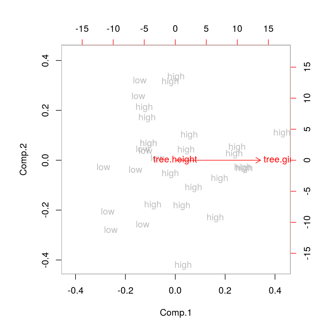

We see that trees high in volume tend to have a high tree girth, but the three height doesn’t give any information on tree volume. This is likely wrong and the consequence of the two different unit measures.

We could use the same units, or we could standardize the variables. I expect both will lead to a more balanced picture of the variability. Of course in this case one can argue that the variables should have the same unit but not be standardized, which may be a valid argument, were it not that we are measuring two different things. (When we would be measuring the weight of the tree and the girth of the tree, the scale on which both should be measured is no longer very clear. In this case we have a clear argument to work on the standardized variables.)

tree.height<-tree.height*5280
tree<-cbind(tree.height,tree.girth)

#do the PCA
tree.pca<-princomp(tree)
summary(tree.pca)

## Importance of components:
##                           Comp.1    Comp.2
## Standard deviation     6.5088696 2.5407042
## Proportion of Variance 0.8677775 0.1322225
## Cumulative Proportion  0.8677775 1.0000000

loadings(tree.pca)

## 
## Loadings:
##             Comp.1 Comp.2
## tree.height  0.956  0.293
## tree.girth   0.293 -0.956
## 
##                Comp.1 Comp.2
## SS loadings       1.0    1.0
## Proportion Var    0.5    0.5
## Cumulative Var    0.5    1.0

biplot(tree.pca,xlabs=tree.vol,col=c("grey","red"))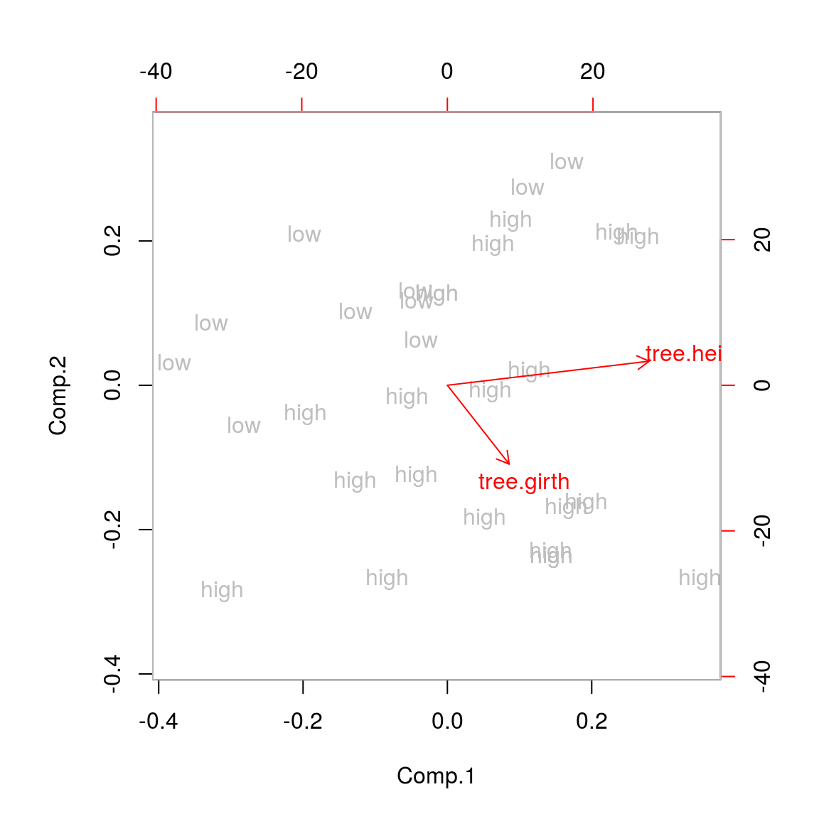

We now see that trees which are tall and have a big girth, are high in volume (bottom left corner), compared to low girth and low height for low volume trees (upper right corner). This intuitively makes sense.

If one watches closely, however, we see that the contrast between high/low volume is strongest in the girth direction and not in the height direction. Let’s see what happens when we standardize:

tree<-scale(tree,center=F,scale=T)
tree.pca<-princomp(tree)
summary(tree.pca)

## Importance of components:
##                           Comp.1     Comp.2
## Standard deviation     0.2275561 0.06779544
## Proportion of Variance 0.9184749 0.08152510
## Cumulative Proportion  0.9184749 1.00000000

loadings(tree.pca)

## 
## Loadings:
##             Comp.1 Comp.2
## tree.height  0.203  0.979
## tree.girth   0.979 -0.203
## 
##                Comp.1 Comp.2
## SS loadings       1.0    1.0
## Proportion Var    0.5    0.5
## Cumulative Var    0.5    1.0

biplot(tree.pca,xlabs=tree.vol,col=c("grey","red"))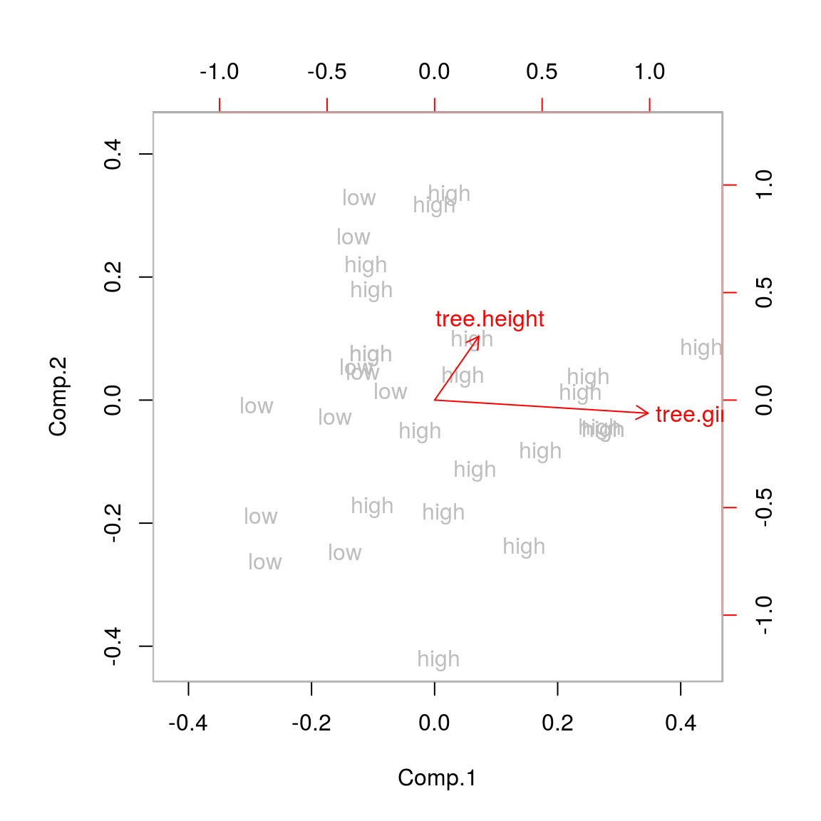

Indeed, the girth now explains the majority of the difference in high and low volume trees! (The length of the arrow in the biplot is indicatory of the variance in the original variable.) So even if things are measured on the same scale, standardizing may be useful. Not standardizing may be recommended when we are for example comparing the length of different species of trees because this is exactly the same measurement.