15 Random forest

15.1 Practical experiments

15.1.1 Random forest for prediction of iris

The caret package (short for _C_lassification _A_nd _RE_gression _T_raining) is a set of functions that attempt to streamline the process for creating predictive models. The package contains tools for:

data splitting
pre-processing
feature selection
model tuning using resampling
variable importance estimation

15.1.1.1 Required R packages

Required packages:

caret   
AppliedPredictiveModeling 
ellipse

Attribute Information:

sepal length in cm
sepal width in cm
petal length in cm
petal width in cm
class:

– Iris Setosa – Iris Versicolour – Iris Virginica

str(iris)

## 'data.frame':    150 obs. of  5 variables:
##  $ Sepal.Length: num  5.1 4.9 4.7 4.6 5 5.4 4.6 5 4.4 4.9 ...
##  $ Sepal.Width : num  3.5 3 3.2 3.1 3.6 3.9 3.4 3.4 2.9 3.1 ...
##  $ Petal.Length: num  1.4 1.4 1.3 1.5 1.4 1.7 1.4 1.5 1.4 1.5 ...
##  $ Petal.Width : num  0.2 0.2 0.2 0.2 0.2 0.4 0.3 0.2 0.2 0.1 ...
##  $ Species     : Factor w/ 3 levels "setosa","versicolor",..: 1 1 1 1 1 1 1 1 1 1 ...

head(iris)

##   Sepal.Length Sepal.Width Petal.Length Petal.Width Species
## 1          5.1         3.5          1.4         0.2  setosa
## 2          4.9         3.0          1.4         0.2  setosa
## 3          4.7         3.2          1.3         0.2  setosa
## 4          4.6         3.1          1.5         0.2  setosa
## 5          5.0         3.6          1.4         0.2  setosa
## 6          5.4         3.9          1.7         0.4  setosa

dim(iris)

## [1] 150   5

15.1.1.2 Visulization

15.1.1.2.1 Scatterplot Matrix

#install.packages("AppliedPredictiveModeling")
library(AppliedPredictiveModeling)
transparentTheme(trans = .4)
#install.packages("caret")
library(caret)

## 
## Attaching package: 'caret'

## The following object is masked from 'package:survival':
## 
##     cluster

featurePlot(x = iris[, 1:4], 
            y = iris$Species, 
            plot = "pairs",
            ## Add a key at the top
            auto.key = list(columns = 3))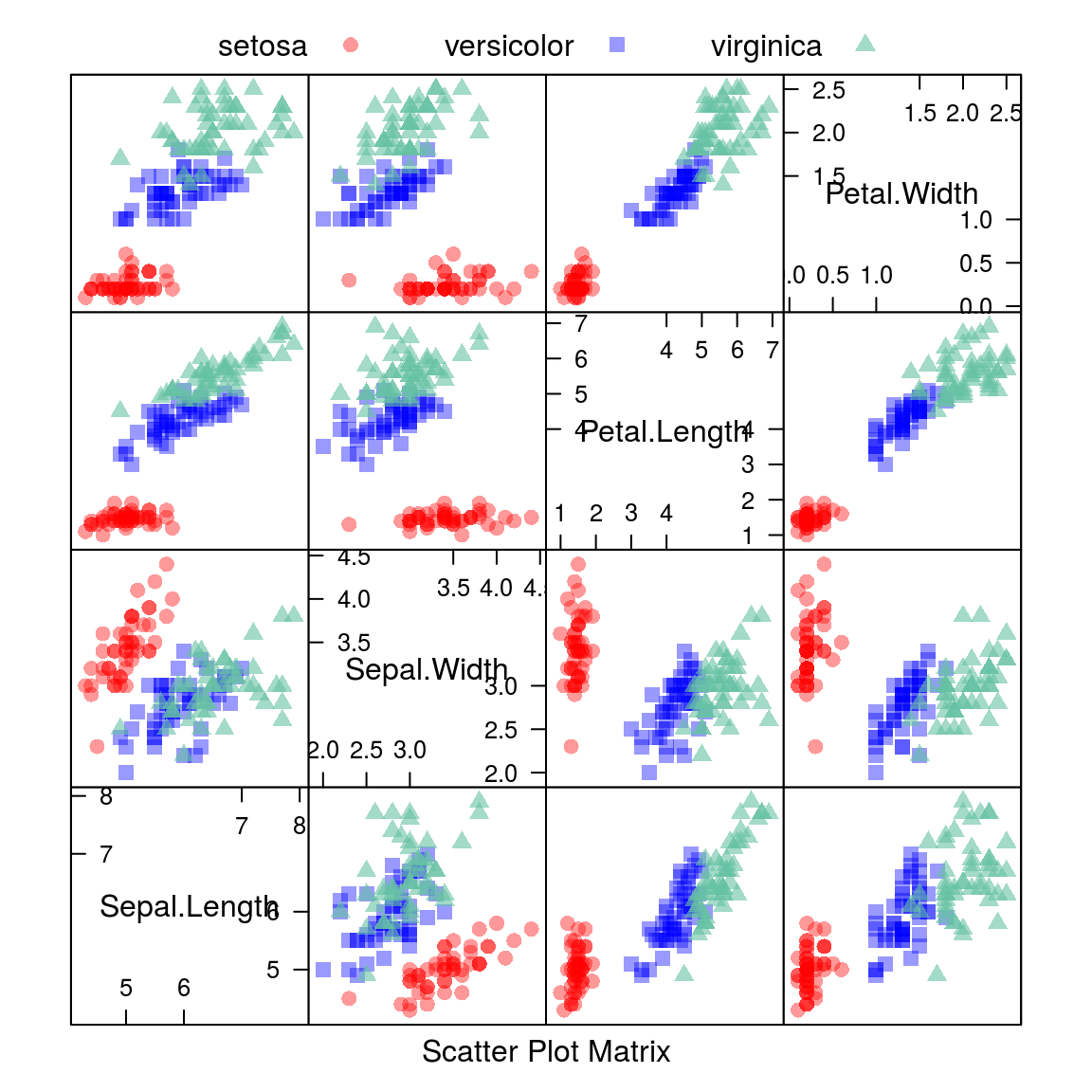

15.1.1.2.2 Scatterplot Matrix with Ellipses

#install.packages("ellipse")
library(ellipse)

## 
## Attaching package: 'ellipse'

## The following object is masked from 'package:graphics':
## 
##     pairs

featurePlot(x = iris[, 1:4], 
            y = iris$Species, 
            plot = "ellipse",
            ## Add a key at the top
            auto.key = list(columns = 3))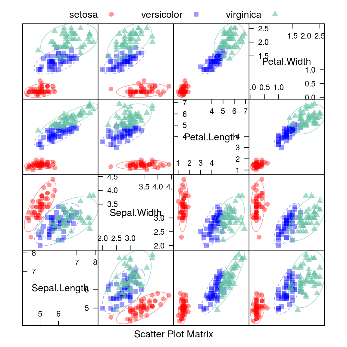

15.1.1.2.3 Overlayed Density Plots

featurePlot(x = iris[, 1:4], 
            y = iris$Species,
            plot = "density", 
            ## Pass in options to xyplot() to 
            ## make it prettier
            scales = list(x = list(relation="free"), 
                          y = list(relation="free")), 
            adjust = 1.5, 
            pch = "|", 
            layout = c(4, 1), 
            auto.key = list(columns = 3))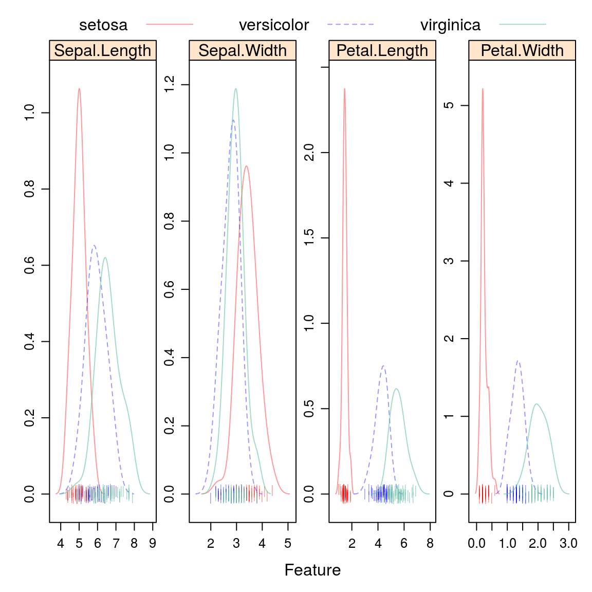

15.1.1.2.4 Box Plots

featurePlot(x = iris[, 1:4], 
            y = iris$Species, 
            plot = "box", 
            ## Pass in options to bwplot() 
            scales = list(y = list(relation="free"),
                          x = list(rot = 90)),  
            layout = c(4,1 ), 
            auto.key = list(columns = 2))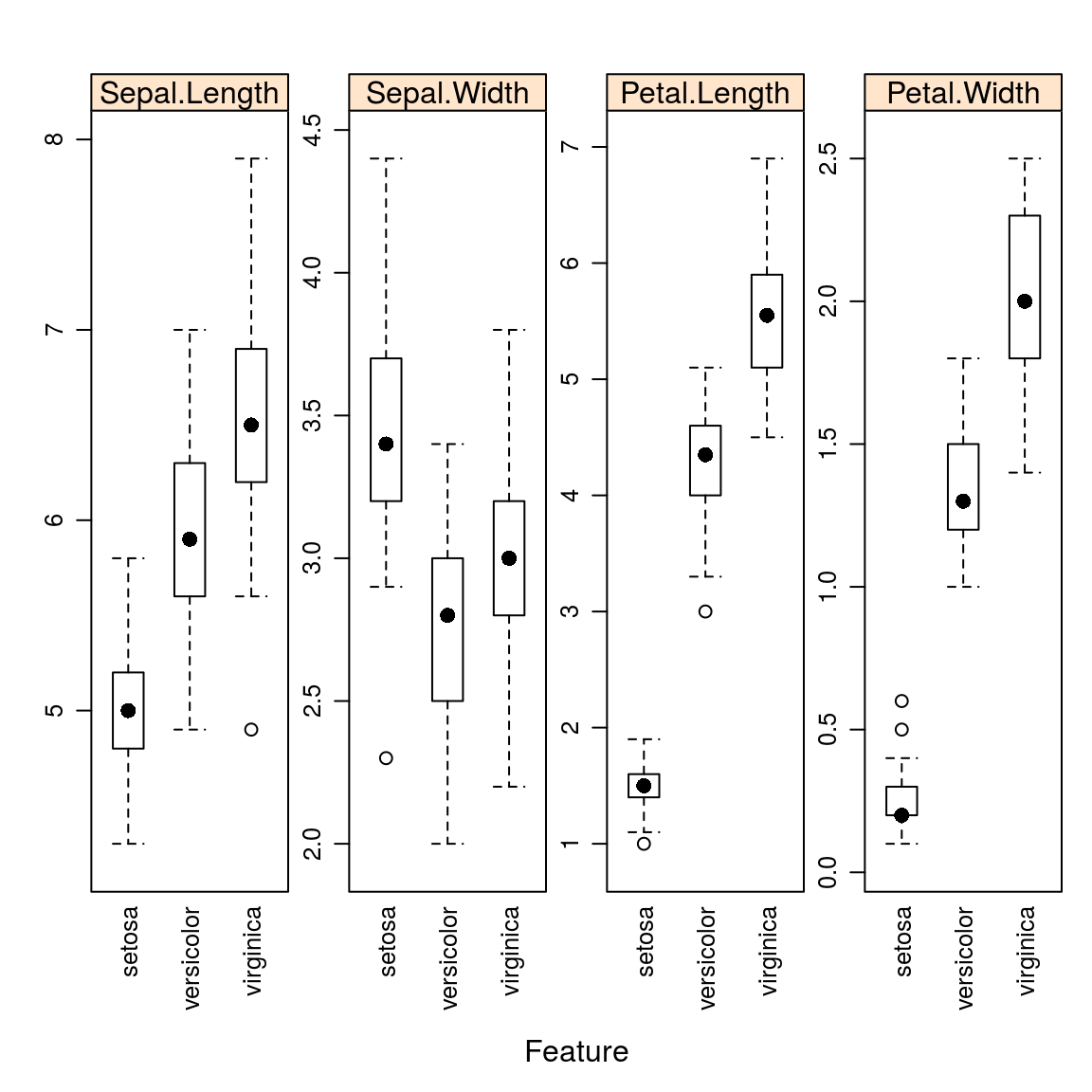

15.1.1.2.5 Machine leraning - Random forest

15.1.1.2.6 Model Train

set.seed(186)
# Data Splitting
train_index <- createDataPartition(iris$Species, p = 0.75, , times=1, list = FALSE)
train_set = iris[train_index, ]
test_set  = iris[-train_index, ]
fit_rf_cv <- train(Species ~ ., data=train_set, method='rf', metric = "Accuracy",
                   trControl=trainControl(method="cv",number=5)) 
fit_rf_cv

## Random Forest 
## 
## 114 samples
##   4 predictor
##   3 classes: 'setosa', 'versicolor', 'virginica' 
## 
## No pre-processing
## Resampling: Cross-Validated (5 fold) 
## Summary of sample sizes: 91, 91, 93, 91, 90 
## Resampling results across tuning parameters:
## 
##   mtry  Accuracy   Kappa    
##   2     0.9398551  0.9100274
##   3     0.9398551  0.9100274
##   4     0.9398551  0.9100274
## 
## Accuracy was used to select the optimal model using the largest value.
## The final value used for the model was mtry = 2.

## Variance importance
rfVarImpcv = varImp(fit_rf_cv)
rfVarImpcv

## rf variable importance
## 
##              Overall
## Petal.Width   100.00
## Petal.Length   95.11
## Sepal.Length   16.93
## Sepal.Width     0.00

15.1.1.2.7 Testing test data

## predict
test_set$predict_rf <- predict(fit_rf_cv, test_set, "raw")
confusionMatrix(test_set$predict_rf, test_set$Species)

## Confusion Matrix and Statistics
## 
##             Reference
## Prediction   setosa versicolor virginica
##   setosa         12          0         0
##   versicolor      0         11         1
##   virginica       0          1        11
## 
## Overall Statistics
##                                           
##                Accuracy : 0.9444          
##                  95% CI : (0.8134, 0.9932)
##     No Information Rate : 0.3333          
##     P-Value [Acc > NIR] : 1.728e-14       
##                                           
##                   Kappa : 0.9167          
##                                           
##  Mcnemar's Test P-Value : NA              
## 
## Statistics by Class:
## 
##                      Class: setosa Class: versicolor Class: virginica
## Sensitivity                 1.0000            0.9167           0.9167
## Specificity                 1.0000            0.9583           0.9583
## Pos Pred Value              1.0000            0.9167           0.9167
## Neg Pred Value              1.0000            0.9583           0.9583
## Prevalence                  0.3333            0.3333           0.3333
## Detection Rate              0.3333            0.3056           0.3056
## Detection Prevalence        0.3333            0.3333           0.3333
## Balanced Accuracy           1.0000            0.9375           0.9375