Chapter 23 Basic statistics - Descriptive Statistics
23.1 Probability distribution
23.1.1 Geometirc distribution
The geometric distribution is the distribution of the number of trials needed to get get the first success in repeated independent Bernolli trails.
23.1.2 Bionomial distribution
The binomial distribution is the distribution of the number of successes (X) in a fixed number (n) if independent Bernolli trails.
23.1.3 Negative binomial distribution
The negative bionomial distribution distribution is the distribution of the number of trials needed (X) to get the _r_th success (r)(jbstatistics (2012)).
\[ \left(\begin{array}{l} {x-1} \\ {r-1} \end{array}\right) p^{r-1}(1-p)^{(x-1)-(r-1)} \]
The probabilty of the rth success that occures on the xth trial is:
\[ \begin{aligned} P(X=x) &=p \times\left(\begin{array}{c} {x-1} \\ {r-1} \end{array}\right) p^{r-1}(1-p)^{(x-1)-(r-1)} \\ &=\left(\begin{array}{c} {x-1} \\ {r-1} \end{array}\right) p^{r}(1-p)^{x-r} \end{aligned} \]
We say Random varaible X is distributed \[X \sim N B(r, p)\]. The mean is: \[\mu=\frac{r}{p}\]. The variance is \[\sigma^{2}=\frac{r(1-p)}{p^{2}}\].
X is the count of independent Bernoulli trials required to achieve the rth successful trial when the probability of success is constant p.
R function dnbinom gives the density. dnbbinom(x, size, prob) calculate the probability that a number of failures x occurs before r-th success, in a sequence of Bernoulli trials, for which the probability of individual success is p.
An oil company has a p = 0.20 chance of striking oil when drilling a well. What is the probability the company drills x = 7 wells to strike oil r = 3 times?
r = 3
p = 0.20
n = 7 - r
# exact
dnbinom(x = n, size = r, prob = p)
## [1] 0.049152# simulated
mean(rnbinom(n = 10000, size = r, prob = p) == n)## [1] 0.0497barplot(dnbinom(1:25,2,0.5), col="grey", names.arg=1:25)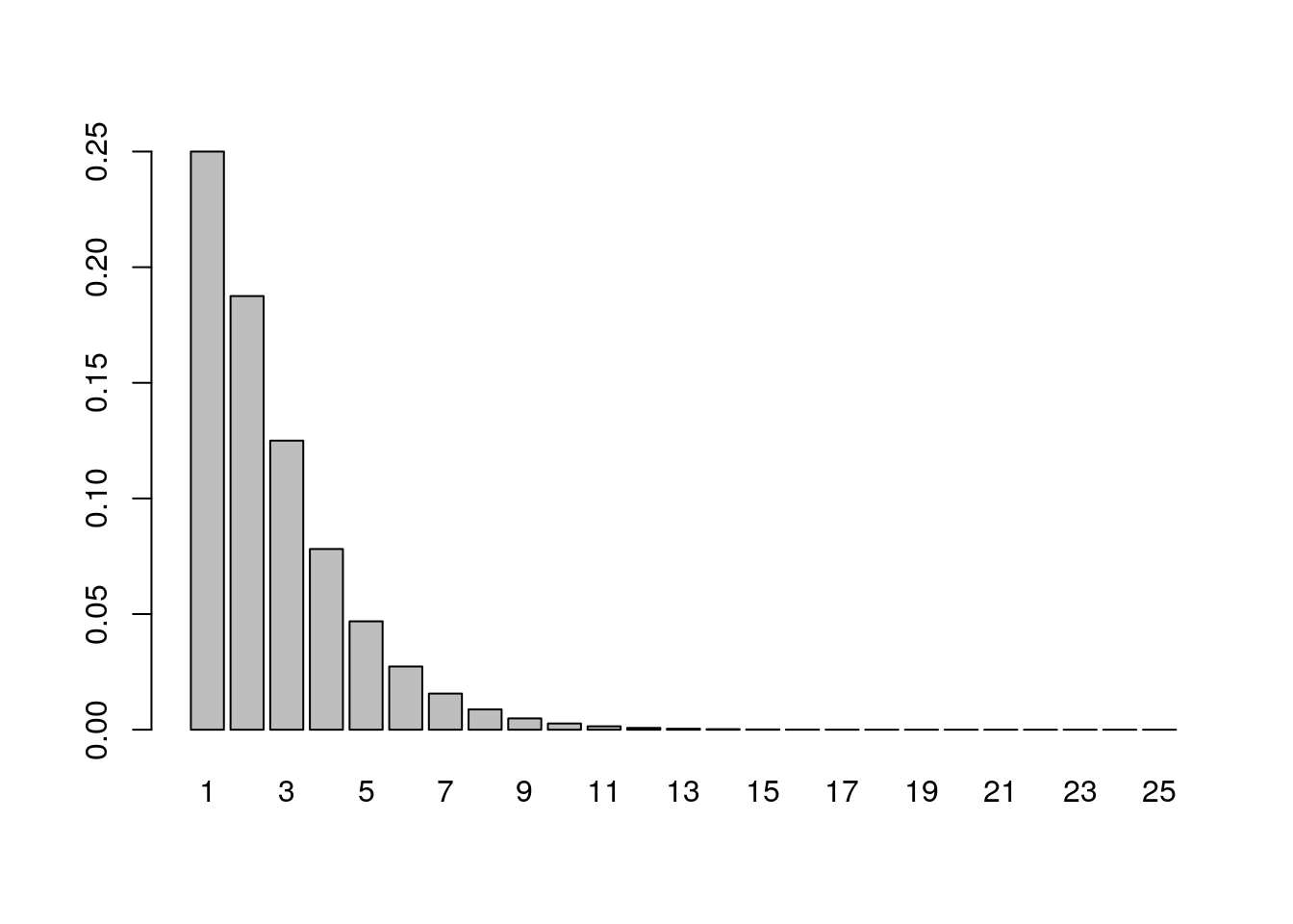
suppressPackageStartupMessages(library(dplyr))
suppressPackageStartupMessages(library(ggplot2))

data.frame(x = 0:10, prob = dnbinom(x = 0:10, size = r, prob = p)) %>%
  mutate(Failures = ifelse(x == n, n, "other")) %>%
ggplot(aes(x = factor(x), y = prob, fill = Failures)) +
  geom_col() +
  geom_text(
    aes(label = round(prob,2), y = prob + 0.01),
    position = position_dodge(0.9),
    size = 3,
    vjust = 0
  ) +
  labs(title = "Probability of r = 3 Successes in X = 7 Trials",
       subtitle = "NB(3,.2)",
       x = "Failed Trials (X - r)",
y = "Probability") 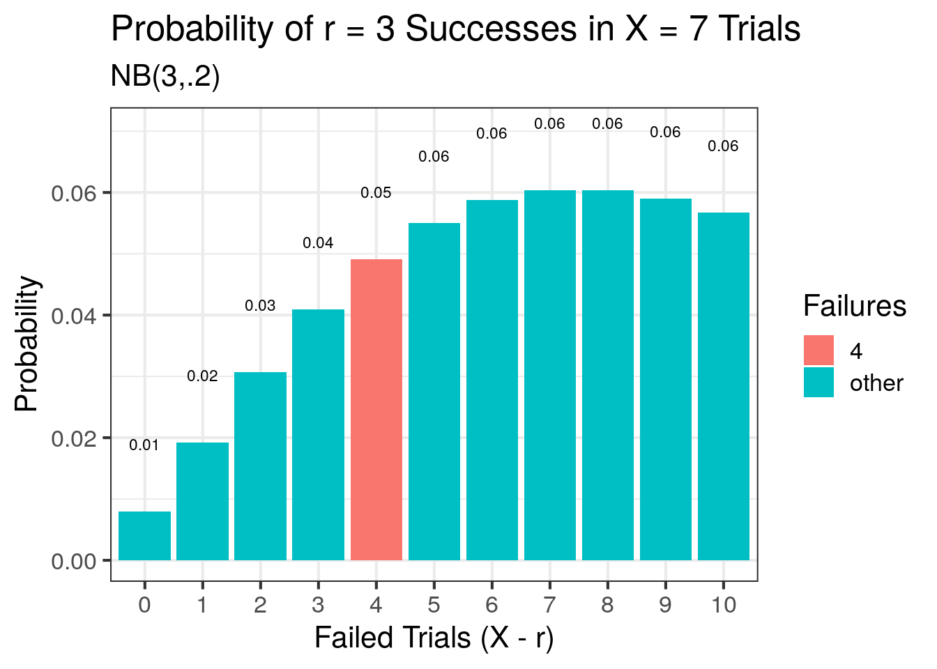
#What is the expected number of trials to achieve r = 3 successes when the probability of success is p = 0.2?
r = 3
p = 0.20
# mean
# exact
r / p
## [1] 15# simulated
mean(rnbinom(n = 10000, size = 3, prob = p)) + r## [1] 14.9638# Variance
# exact
r * (1 - p) / p^2## [1] 60# simulated
var(rnbinom(n = 100000, size = r, prob = p))## [1] 60.21857suppressPackageStartupMessages(library(dplyr))
suppressPackageStartupMessages(library(ggplot2))
data.frame(x = 1:20,
pmf = dnbinom(x = 1:20, size = r, prob = p),
cdf = pnbinom(q = 1:20, size = r, prob = p, lower.tail = TRUE)) %>%
ggplot(aes(x = factor(x), y = cdf)) +
geom_col() +
geom_text(
aes(label = round(cdf,2), y = cdf + 0.01),
position = position_dodge(0.9),
size = 3,
vjust = 0
) +
labs(title = "Cumulative Probability of X = x failed trials to achieve 3rd success",
subtitle = "NB(3,.2)",
x = "Failed Trials (x)",
y = "probability") 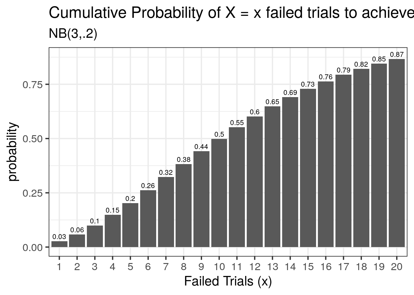
23.1.3.1 Why is it called Negative Binomial?
The “negative” part of negative binomial stems from the fact that one facet of the binomial distribution is reversed: in a binomial experiment, we count the number of successes in a fixed number of trials. In a negative binomial experiment, we’re counting the failures, or how many cards it takes you to pick two aces.