Chapter 13 R introduction

I started to work on

13.1 Basic R function

Data structures are variables with informaton stored in. R operates on these data structures. Numberic vector is a single entity consisting of a collection of numbers.

<- is call assignment operator.

# semi-colon (‘;’) can be removed:
gene1_count <- 100;  
gene1_count

## [1] 100

class(gene1_count)

## [1] "numeric"

gene1_count <- c(100)
gene1_count

## [1] 100

class(gene1_count)

## [1] "numeric"

A semi-colon (;) or a newline are used to separate commands

gene_counts <- c(5, 6, 100, 100, 200)
gene_counts

## [1]   5   6 100 100 200

class(gene_counts)

## [1] "numeric"

gene1_info <- c(6, "TF")
gene1_info

## [1] "6"  "TF"

class(gene1_info)

## [1] "character"

13.2 Producing Simple Graphs with R

The credit of this section goes to Dr. Frank McCown (Frank McCown (2006)).

13.2.1 Line Charts

# Define the gene_expr_level vector with 5 values
gene_expr_level <- c(8, 20, 20, 100, 120)

# Graph the gene_expr_fpkm vector with all defaults
plot(gene_expr_level)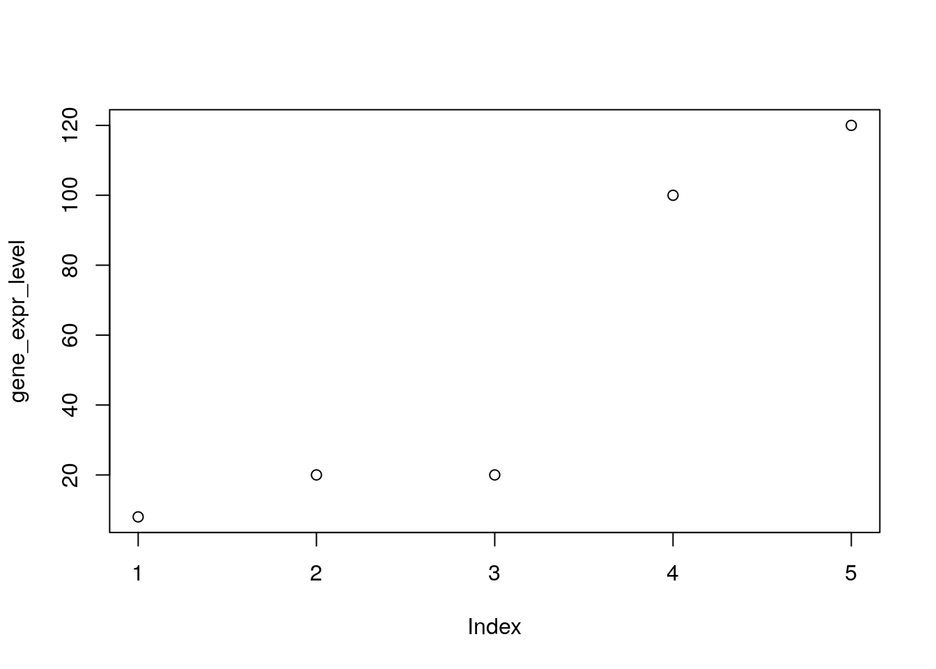

Let’s add a title, a line to connect the points, and some color:

# Define the gene_expr_level vector with 5 values
geneX_expr <- c(8, 20, 20, 100, 120)

# Graph cars using blue points overlayed by a line 
plot(geneX_expr, type="o", col="blue")

# Create a title with a red, bold/italic font
title(main="GeneX", col.main="red", font.main=4)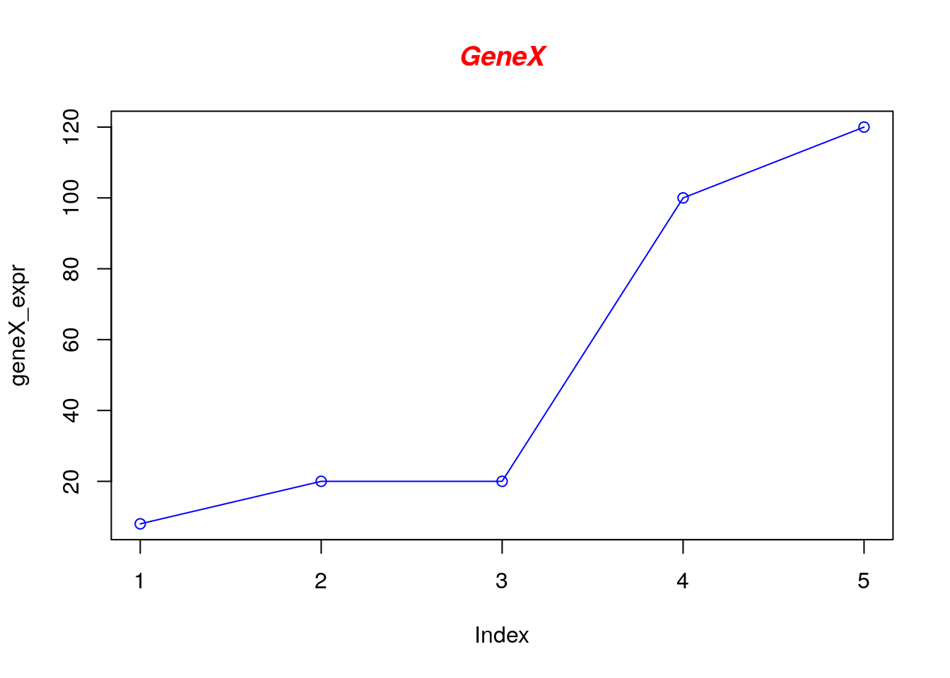

Now let’s add a red line for trucks and specify the y-axis range directly so it will be large enough to fit the truck data:

# Define the gene_expr_level vector with 5 values
geneX_expr <- c(8, 20, 20, 100, 120)
geneY_expr <- c(300, 280, 20, 10, 12)

# Graph cars using blue points overlayed by a line 
plot(geneX_expr, type="o", col="blue", ylim=c(0,300))
# Graph trucks with red dashed line and square points
lines(geneY_expr, type="o", pch=22, lty=2, col="red")
# Create a title with a red, bold/italic font
title(main="Gene expresion level", col.main="red", font.main=4)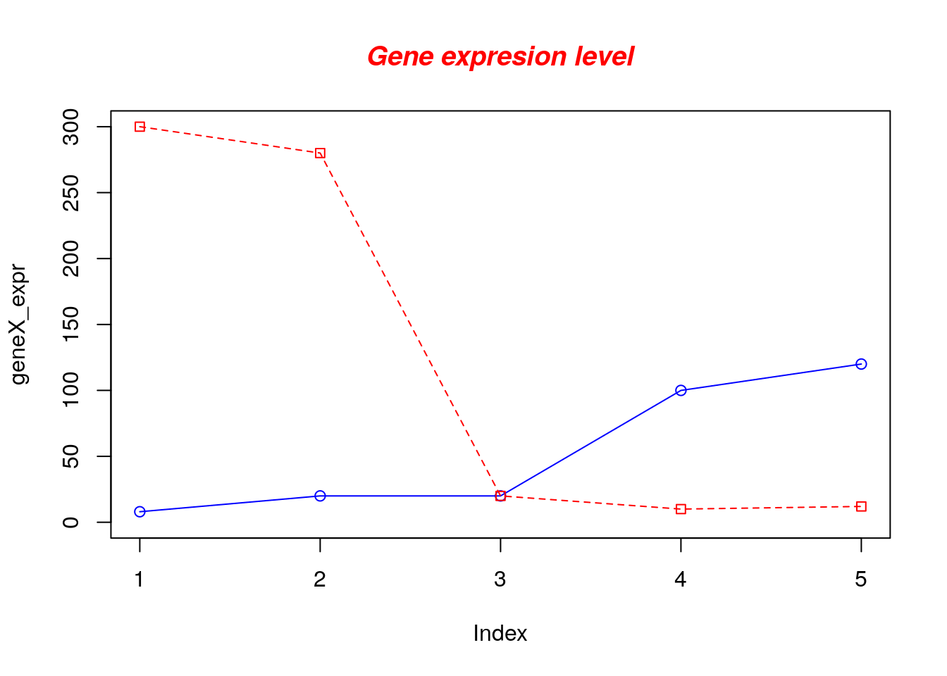

13.3 XXX

fruit = c("apple", "apple", "pear", "orange")
fruit == "apple"

## [1]  TRUE  TRUE FALSE FALSE

fruit = c("apple", "apple", "pear", "orange")
which(fruit == "apple")

## [1] 1 2

fruit = c("apple", "apple", "pear", "orange")
which(fruit == "apple" | fruit == "pear")

## [1] 1 2 3

13.4 Logic `&&` and `|`

The short answer is that && and || only ever return a single (scalar, length-1 vector) TRUE or FALSE value, whereas | and & return a vector after doing element-by-element comparisons.

The only place in R you routinely use a scalar TRUE/FALSE value is in the conditional of an if statement, so you’ll often see && or || used in idioms like:

if (length(x) > 0 && any(is.na(x))) { do.something() }

In most other instances you’ll be working with vectors and use & and | instead.

13.5 List as dictionary

the list type is a good approximation. You can use names() on your list to set and retrieve the ‘keys’:

foo <- vector(mode="list", length=3)
names(foo) <- c("tic", "tac", "toe")
foo[[1]] <- 12; foo[[2]] <- 22; foo[[3]] <- 33
foo

## $tic
## [1] 12
## 
## $tac
## [1] 22
## 
## $toe
## [1] 33

names(foo)

## [1] "tic" "tac" "toe"

13.6 Parsing arguments as string

13.6.1 String as xlim

13.6.2 How to access data frame column using variable

a = "col1"
b = "col2"
d = data.frame(a=c(1,2,3),b=c(4,5,6))
colnames(d) <- c("col1", "col2")
d[[a]]

## [1] 1 2 3

This is useful when you parse a variable from the command line

13.6.3 How to create a formula from a

It can be useful to create a formula from a string. This often occurs in functions where the formula arguments are passed in as strings.

design1 = "diet"
design2 = "age"
## `~ diet + age`
as.formula(paste0("~ " , design1, " + ", design2))

## ~diet + age

cat(readLines('code_R/parse_aug_as.formula.R'), sep = '\n')

argv <- commandArgs(trailingOnly = T)

level1 <- argv[1]
level2 <- argv[2]

#First, build a simple data frame with time as a factor and Time as a continuous,
#numeric variable. The two variables look alike when you print the data frame.
#But, if you summarize the data, you see that they are different.
d <- data.frame(level1 = factor(1:4), level2 = 1:4)
colnames(d)<-c(level1, level2)
summary(d)

Rscript code_R/parse_aug_as.formula.R time Time

##  time       Time     
##  1:1   Min.   :1.00  
##  2:1   1st Qu.:1.75  
##  3:1   Median :2.50  
##  4:1   Mean   :2.50  
##        3rd Qu.:3.25  
##        Max.   :4.00

References

Frank McCown. 2006. Producing Simple Graphs with r. Searcy, AR: Harding University. https://www.harding.edu/fmccown/r/.