Chapter 27 Linear regression
here we will be analyzing the NHANES data, allowing us to illustrate the use of these two regression methods for addressing meaningful questions with actual data.
# Read the 2015-2016 wave of NHANES data
df <- read.csv("data/nhanes_2015_2016.csv")

col2keep <- c("BPXSY1", "RIDAGEYR", "RIAGENDR", "RIDRETH1", "DMDEDUC2", "BMXBMI", "SMQ020")
df_subset <- df[, col2keep]
dim(df_subset)
## [1] 5735 7df_subset <- df_subset[complete.cases(df_subset), ]
dim(df_subset)## [1] 5102 7head(df_subset)## BPXSY1 RIDAGEYR RIAGENDR RIDRETH1 DMDEDUC2 BMXBMI SMQ020
## 1 128 62 1 3 5 27.8 1
## 2 146 53 1 3 3 30.8 1
## 3 138 78 1 3 3 28.8 1
## 4 132 56 2 3 5 42.4 2
## 5 100 42 2 4 4 20.3 2
## 6 116 72 2 1 2 28.6 2We will focus initially on regression models in which systolic blood pressure (SBP) is the outcome (dependent) variable. That is, we will predict SBP from other variables. SBP is an important indicator of cardiovascular health. It tends to increase with age, is greater for overweight people (i.e. people with greater body mass index or BMI), and also differs among demographic groups, for example among gender and ethnic groups.
Since SBP is a quantitative variable, we will model it using linear regression. Linear regression is the most widely-utilized form of statistical regression. While linear regression is commonly used with quantitative outcome variables, it is not the only type of regression model that can be used with quantitative outcomes, nor is it the case that linear regression can only be used with quantitative outcomes. However, linear regression is a good default starting point for any regression analysis using a quantitative outcome variable.
27.1 Interpreting regression parameters in a basic model
We start with a simple linear regression model with only one covariate, age, predicting SBP. In the NHANES data, the variable BPXSY1 contains the first recorded measurement of SBP for a subject, and RIDAGEYR is the subject’s age in years. The model that is fit in the next cell expresses the expected SBP as a linear function of age:
simple.fit = lm(BPXSY1 ~ RIDAGEYR, data=df_subset)

summary(simple.fit)
##
## Call:
## lm(formula = BPXSY1 ~ RIDAGEYR, data = df_subset)
##
## Residuals:
## Min 1Q Median 3Q Max
## -52.355 -10.843 -1.500 8.686 109.162
##
## Coefficients:
## Estimate Std. Error t value Pr(>|t|)
## (Intercept) 102.09352 0.68464 149.1 <2e-16 ***
## RIDAGEYR 0.47585 0.01304 36.5 <2e-16 ***
## ---
## Signif. codes: 0 '***' 0.001 '**' 0.01 '*' 0.05 '.' 0.1 ' ' 1
##
## Residual standard error: 16.46 on 5100 degrees of freedom
## Multiple R-squared: 0.2072, Adjusted R-squared: 0.207
## F-statistic: 1333 on 1 and 5100 DF, p-value: < 2.2e-16Much of the output above is not relevant for us, so focus on the center section of the output where the header begins with Coefficients. This section contains the estimated values of the parameters of the regression model, their standard errors, and other values that are used to quantify the uncertainty in the regression parameter estimates. Note that the parameters of a regression model, which appear in the column labeled coef in the table above, may also be referred to as slopes or effects.
This fitted model implies that when
comparing two people whose ages differ by one year, the older person
will on average have 0.48 units higher SBP than the younger person.
This difference is statistically significant, based on the p-value
shown under the column labeled Pr(>|t|). This means that there
is strong evidence that there is a real association between between systolic blood
pressure and age in this population.
SBP is measured in units of millimeters of mercury, expressed mm/Hg. In order to better understand the meaning of the estimated regression parameter 0.48, we can look at the standard deviation of SBP:
sd(df_subset$BPXSY1)## [1] 18.48656The standard deviation of around 18.5 is large compared to the
regression slope of 0.48. However the regression slope corresponds to
the average change in SBP for a single year of age, and this effect
accumulates with age. Comparing a 40 year-old person to a 60 year-old
person, there is a 20 year difference in age, which translates into a
20 * 0.48 = 9.6 unit difference in average SBP between these two
people. This difference is around half of one standard deviation, and
would generally be considered to be an important and meaningful shift.
27.1.1 R-squared and correlation
In the case of regression with a
single independent variable, as we have here, there is a very close
correspondence between the regression analysis and a Pearson
correlation analysis.
The primary summary statistic for assessing the strength of a
predictive relationship in a regression model is the R-squared, which is
shown to be 0.207 in the regression output above. This means that 21%
of the variation in SBP is explained by age. Note that this value is
exactly the same as the squared Pearson correlation coefficient
between SBP and age, as shown below.
cor.test(df_subset$BPXSY1, df_subset$RIDAGEYR)##
## Pearson's product-moment correlation
##
## data: df_subset$BPXSY1 and df_subset$RIDAGEYR
## t = 36.504, df = 5100, p-value < 2.2e-16
## alternative hypothesis: true correlation is not equal to 0
## 95 percent confidence interval:
## 0.4331109 0.4766303
## sample estimates:
## cor
## 0.4551424plot(BPXSY1 ~ RIDAGEYR, data = df_subset)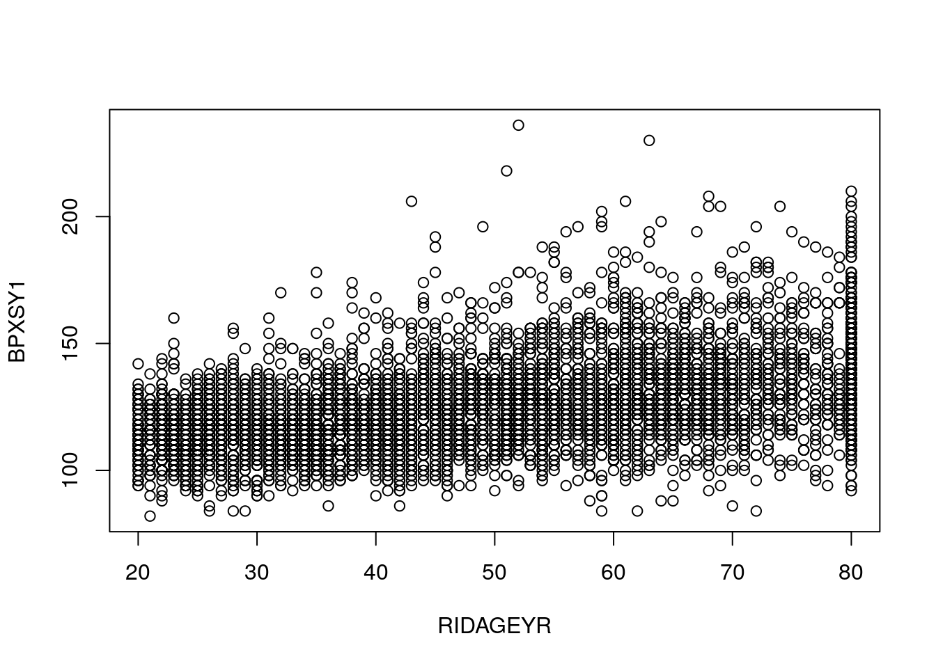
27.2 Reference
Coursera classes