Chapter 15 Heatmap Tutorial

15.1 Install `pheatmap` package

install.packages("pheatmap")

15.2 Draw a heatmap for gene expression of RNA-seq data

library(pheatmap)
gene_exp <- read.table("data/maize_embryo_specific_gene_Sheet1.tsv", header=T, row.names=1)
pheatmap(gene_exp)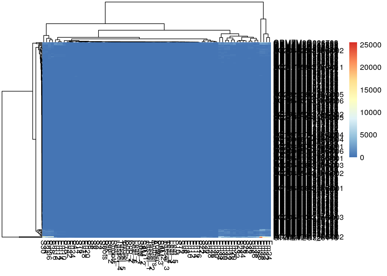

library(ggplot2)
# Set the theme for all the following plots.
theme_set(theme_bw(base_size = 16))

dat <- data.frame(values = as.numeric(unlist(gene_exp)))
summary(dat)

##      values        
##  Min.   :    0.00  
##  1st Qu.:    0.00  
##  Median :    0.40  
##  Mean   :   38.91  
##  3rd Qu.:    6.22  
##  Max.   :25534.25

ggplot(dat, aes(values)) + geom_density(bw = "SJ") + xlim(c(0,100))

## Warning: Removed 958 rows containing non-finite values (stat_density).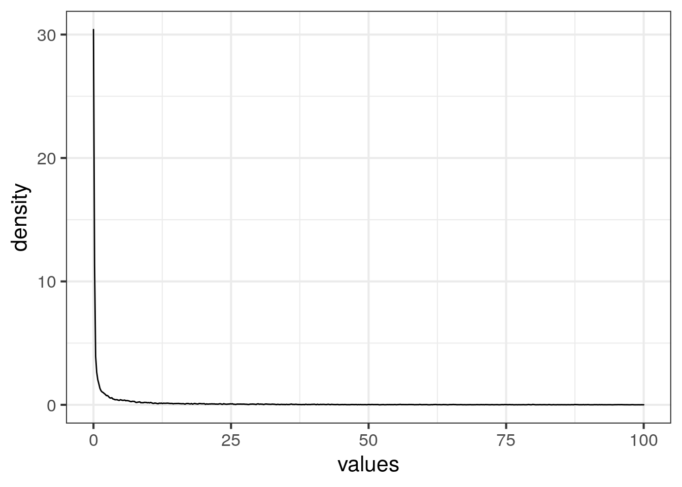

The data is skewed.

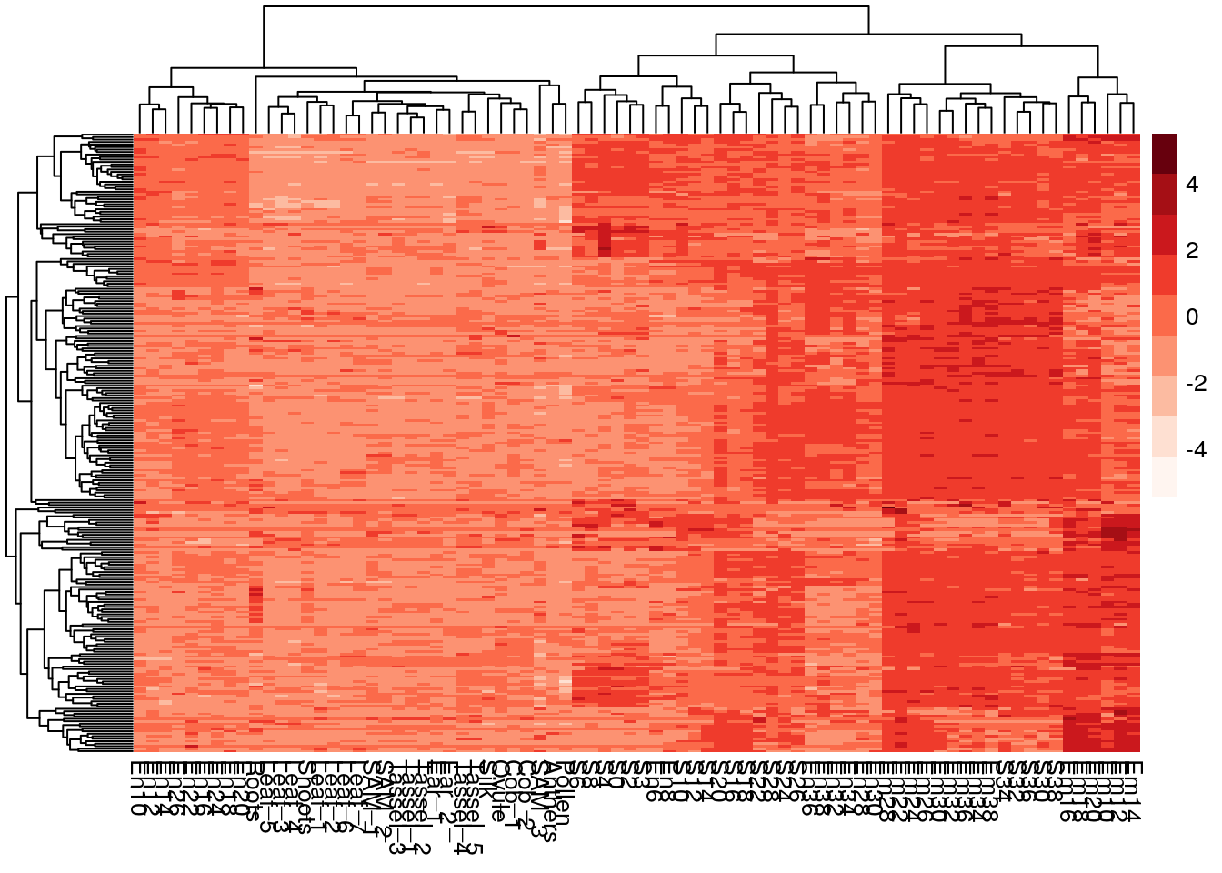
pheatmap(log2(gene_exp + 0.000001), scale="row")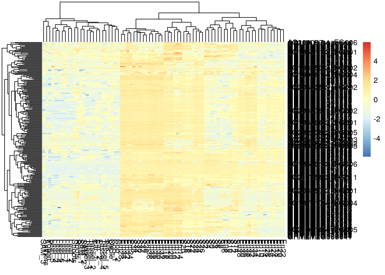

pheatmap(log2(gene_exp + 0.01), scale="row", show_rownames = T, show_colnames = F)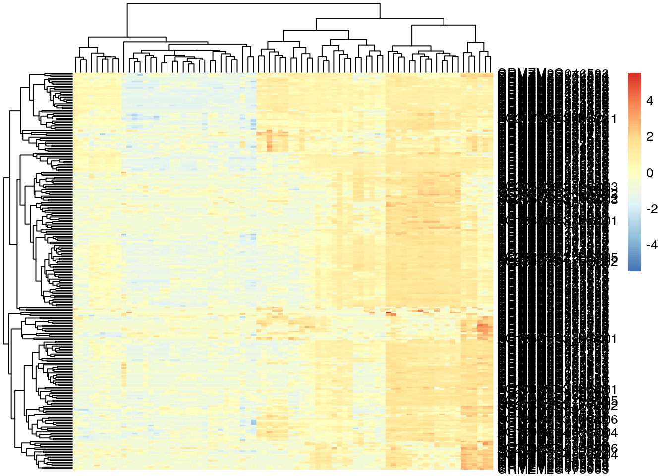

pheatmap(log2(gene_exp + 0.01), scale="row", show_rownames = F, show_colnames = T)

15.3 Add the annotation

15.4

15.5 Transfrom the data

pheatmap(log2(gene_exp + 0.01), show_rownames = F)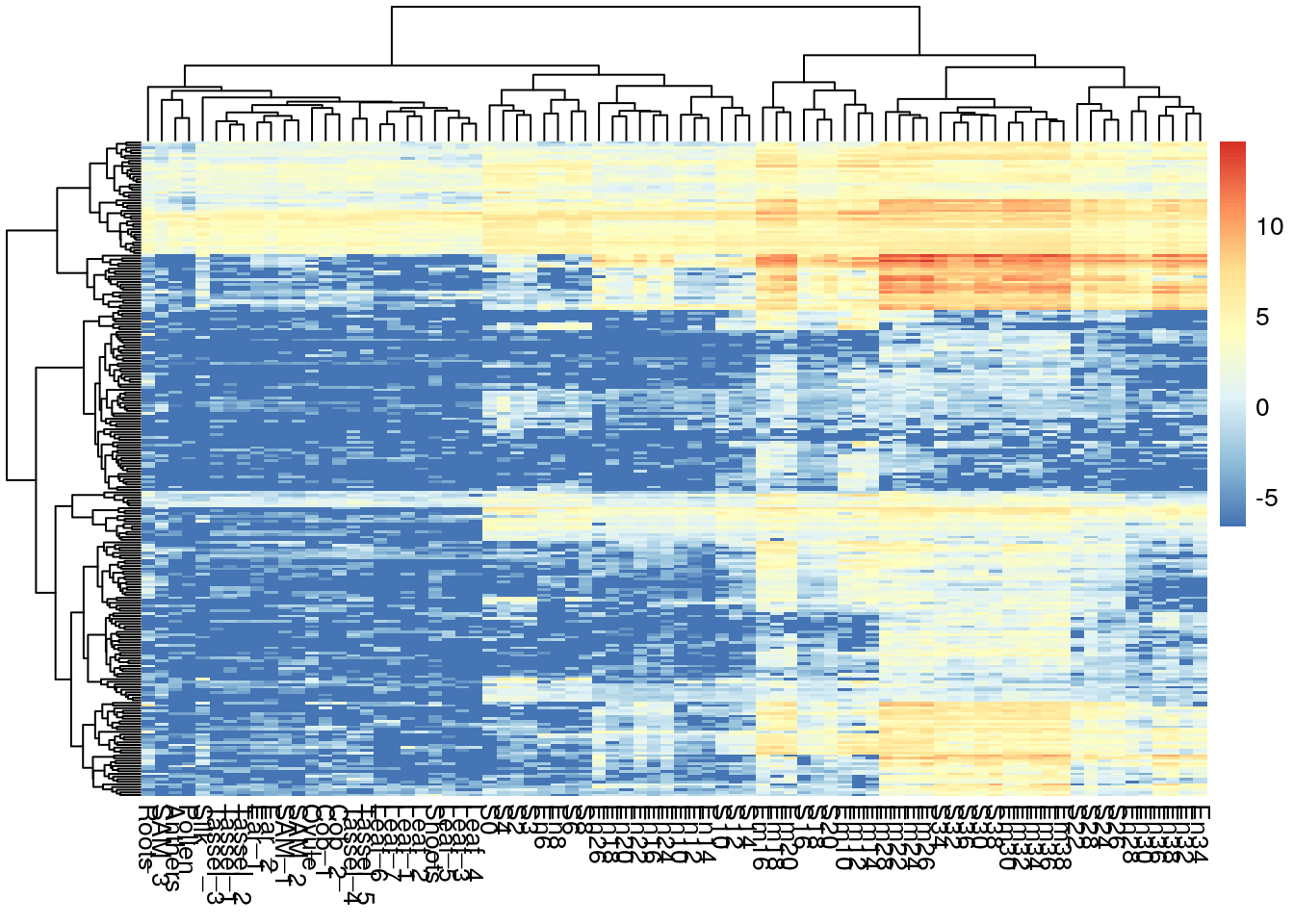

15.6 How to add annotations

15.7 How to cut the trees

15.8 How to get the cluster information from the heatmap

15.9 Change color

15.9.1 Use Brewer

col.pal <- RColorBrewer::brewer.pal(9, "Reds")
col.pal

## [1] "#FFF5F0" "#FEE0D2" "#FCBBA1" "#FC9272" "#FB6A4A" "#EF3B2C" "#CB181D"
## [8] "#A50F15" "#67000D"

pheatmap(log2(gene_exp + 0.01), scale="row",
         show_rownames = F, show_colnames = T)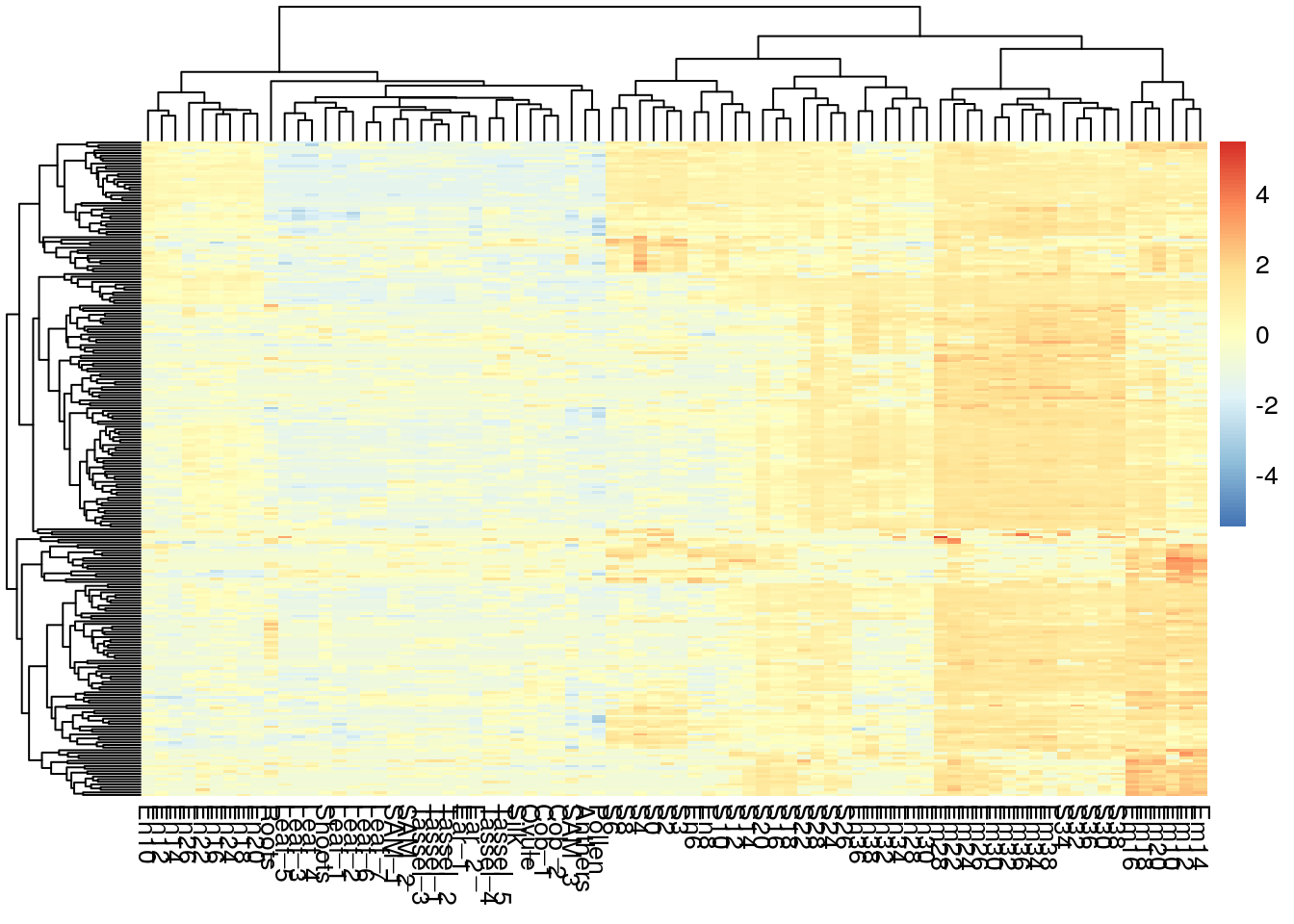

pheatmap(log2(gene_exp + 0.01), scale="row", color = col.pal,
         show_rownames = F, show_colnames = T)