第 5 章 Linear Models
Many of the models we use in data analysis can be presented using matrix algebra. We refer to these types of models as linear models. “Linear” here does not refer to lines, but rather to linear combinations. The representations we describe are convenient because we can write models more succinctly and we have the matrix algebra mathematical machinery to facilitate computation. In this chapter, we will describe in some detail how we use matrix algebra to represent and fit.
In this book, we focus on linear models that represent dichotomous groups: treatment versus control, for example. The effect of diet on mice weights is an example of this type of linear model. Here we describe slightly more complicated models, but continue to focus on dichotomous variables.
As we learn about linear models, we need to remember that we are still working with random variables. This means that the estimates we obtain using linear models are also random variables. Although the mathematics is more complex, the concepts we learned in previous chapters apply here. We begin with some exercises to review the concept of random variables in the context of linear models.
5.1 The Design Matrix
Here we will show how to use the two R functions, formula and model.matrix, in order to produce design matrices (also known as model matrices) for a variety of linear models. For example, in the mouse diet examples we wrote the model as
\[ Y_i = \beta_0 + \beta_1 x_i + \varepsilon_i, i=1,\dots,N \]
with \(Y_i\) the weights and \(x_i\) equal to 1 only when mouse \(i\) receives the high fat diet. We use the term experimental unit to \(N\) different entities from which we obtain a measurement. In this case, the mice are the experimental units.
This is the type of variable we will focus on in this chapter. We call them indicator variables since they simply indicate if the experimental unit had a certain characteristic or not. As we described earlier, we can use linear algebra to represent this model:
\[ \mathbf{Y} = \begin{pmatrix} Y_1\\ Y_2\\ \vdots\\ Y_N \end{pmatrix} , \mathbf{X} = \begin{pmatrix} 1&x_1\\ 1&x_2\\ \vdots\\ 1&x_N \end{pmatrix} , \boldsymbol{\beta} = \begin{pmatrix} \beta_0\\ \beta_1 \end{pmatrix} \mbox{ and } \boldsymbol{\varepsilon} = \begin{pmatrix} \varepsilon_1\\ \varepsilon_2\\ \vdots\\ \varepsilon_N \end{pmatrix} \]
as:
\[ \, \begin{pmatrix} Y_1\\ Y_2\\ \vdots\\ Y_N \end{pmatrix} = \begin{pmatrix} 1&x_1\\ 1&x_2\\ \vdots\\ 1&x_N \end{pmatrix} \begin{pmatrix} \beta_0\\ \beta_1 \end{pmatrix} + \begin{pmatrix} \varepsilon_1\\ \varepsilon_2\\ \vdots\\ \varepsilon_N \end{pmatrix} \]
or simply:
\[ \mathbf{Y}=\mathbf{X}\boldsymbol{\beta}+\boldsymbol{\varepsilon} \]
The design matrix is the matrix \(\mathbf{X}\).
Once we define a design matrix, we are ready to find the least squares estimates. We refer to this as fitting the model. For fitting linear models in R, we will directly provide a formula to the lm function. In this script, we will use the model.matrix function, which is used internally by the lm function. This will help us to connect the R formula with the matrix \(\mathbf{X}\). It will therefore help us interpret the results from lm.
5.1.0.1 Choice of design
The choice of design matrix is a critical step in linear modeling since it encodes which coefficients will be fit in the model, as well as the inter-relationship between the samples. A common misunderstanding is that the choice of design follows straightforward from a description of which samples were included in the experiment. This is not the case. The basic information about each sample (whether control or treatment group, experimental batch, etc.) does not imply a single ‘correct’ design matrix. The design matrix additionally encodes various assumptions about how the variables in \(\mathbf{X}\) explain the observed values in \(\mathbf{Y}\), on which the investigator must decide.
For the examples we cover here, we use linear models to make comparisons between different groups. Hence, the design matrices that we ultimately work with will have at least two columns: an intercept column, which consists of a column of 1’s, and a second column, which specifies which samples are in a second group. In this case, two coefficients are fit in the linear model: the intercept, which represents the population average of the first group, and a second coefficient, which represents the difference between the population averages of the second group and the first group. The latter is typically the coefficient we are interested in when we are performing statistical tests: we want to know if there is a difference between the two groups.
We encode this experimental design in R with two pieces. We start with a formula with the tilde symbol ~. This means that we want to model the observations using the variables to the right of the tilde. Then we put the name of a variable, which tells us which samples are in which group.
Let’s try an example. Suppose we have two groups, control and high fat diet, with two samples each. For illustrative purposes, we will code these with 1 and 2 respectively. We should first tell R that these values should not be interpreted numerically, but as different levels of a factor. We can then use the paradigm ~ group to, say, model on the variable group.
group <- factor( c(1,1,2,2) )
model.matrix(~ group)
## (Intercept) group2
## 1 1 0
## 2 1 0
## 3 1 1
## 4 1 1
## attr(,"assign")
## [1] 0 1
## attr(,"contrasts")
## attr(,"contrasts")$group
## [1] "contr.treatment"(Don’t worry about the attr lines printed beneath the matrix. We won’t be using this information.)
What about the formula function? We don’t have to include this. By starting an expression with ~, it is equivalent to telling R that the expression is a formula:
model.matrix(formula(~ group))## (Intercept) group2
## 1 1 0
## 2 1 0
## 3 1 1
## 4 1 1
## attr(,"assign")
## [1] 0 1
## attr(,"contrasts")
## attr(,"contrasts")$group
## [1] "contr.treatment"What happens if we don’t tell R that group should be interpreted as a factor?
group <- c(1,1,2,2)
model.matrix(~ group)
## (Intercept) group
## 1 1 1
## 2 1 1
## 3 1 2
## 4 1 2
## attr(,"assign")
## [1] 0 1This is not the design matrix we wanted, and the reason is that we provided a numeric variable as opposed to an indicator to the formula and model.matrix functions, without saying that these numbers actually referred to different groups. We want the second column to have only 0 and 1, indicating group membership.
A note about factors: the names of the levels are irrelevant to model.matrix and lm. All that matters is the order. For example:
group <- factor(c("control","control","highfat","highfat"))
model.matrix(~ group)
## (Intercept) grouphighfat
## 1 1 0
## 2 1 0
## 3 1 1
## 4 1 1
## attr(,"assign")
## [1] 0 1
## attr(,"contrasts")
## attr(,"contrasts")$group
## [1] "contr.treatment"produces the same design matrix as our first code chunk.
5.1.0.2 More groups
Using the same formula, we can accommodate modeling more groups. Suppose we have a third diet:
group <- factor(c(1,1,2,2,3,3))
model.matrix(~ group)
## (Intercept) group2 group3
## 1 1 0 0
## 2 1 0 0
## 3 1 1 0
## 4 1 1 0
## 5 1 0 1
## 6 1 0 1
## attr(,"assign")
## [1] 0 1 1
## attr(,"contrasts")
## attr(,"contrasts")$group
## [1] "contr.treatment"Now we have a third column which specifies which samples belong to the third group.
An alternate formulation of design matrix is possible by specifying + 0 in the formula:
group <- factor(c(1,1,2,2,3,3))
model.matrix(~ group + 0)
## group1 group2 group3
## 1 1 0 0
## 2 1 0 0
## 3 0 1 0
## 4 0 1 0
## 5 0 0 1
## 6 0 0 1
## attr(,"assign")
## [1] 1 1 1
## attr(,"contrasts")
## attr(,"contrasts")$group
## [1] "contr.treatment"This group now fits a separate coefficient for each group. We will explore this design in more depth later on.
5.1.0.3 More variables
We have been using a simple case with just one variable (diet) as an example. In the life sciences, it is quite common to perform experiments with more than one variable. For example, we may be interested in the effect of diet and the difference in sexes. In this case, we have four possible groups:
diet <- factor(c(1,1,1,1,2,2,2,2))
sex <- factor(c("f","f","m","m","f","f","m","m"))
table(diet,sex)
## sex
## diet f m
## 1 2 2
## 2 2 2If we assume that the diet effect is the same for males and females (this is an assumption), then our linear model is:
\[ Y_{i}= \beta_0 + \beta_1 x_{i,1} + \beta_2 x_{i,2} + \varepsilon_i \]
To fit this model in R, we can simply add the additional variable with a + sign in order to build a design matrix which fits based on the information in additional variables:
diet <- factor(c(1,1,1,1,2,2,2,2))
sex <- factor(c("f","f","m","m","f","f","m","m"))
model.matrix(~ diet + sex)
## (Intercept) diet2 sexm
## 1 1 0 0
## 2 1 0 0
## 3 1 0 1
## 4 1 0 1
## 5 1 1 0
## 6 1 1 0
## 7 1 1 1
## 8 1 1 1
## attr(,"assign")
## [1] 0 1 2
## attr(,"contrasts")
## attr(,"contrasts")$diet
## [1] "contr.treatment"
##
## attr(,"contrasts")$sex
## [1] "contr.treatment"The design matrix includes an intercept, a term for diet and a term for sex. We would say that this linear model accounts for differences in both the group and condition variables. However, as mentioned above, the model assumes that the diet effect is the same for both males and females. We say these are an additive effect. For each variable, we add an effect regardless of what the other is. Another model is possible here, which fits an additional term and which encodes the potential interaction of group and condition variables. We will cover interaction terms in depth in a later script.
The interaction model can be written in either of the following two formulas:
model.matrix(~ diet + sex + diet:sex)or
model.matrix(~ diet*sex)## (Intercept) diet2 sexm diet2:sexm
## 1 1 0 0 0
## 2 1 0 0 0
## 3 1 0 1 0
## 4 1 0 1 0
## 5 1 1 0 0
## 6 1 1 0 0
## 7 1 1 1 1
## 8 1 1 1 1
## attr(,"assign")
## [1] 0 1 2 3
## attr(,"contrasts")
## attr(,"contrasts")$diet
## [1] "contr.treatment"
##
## attr(,"contrasts")$sex
## [1] "contr.treatment"5.1.0.4 Releveling
The level which is chosen for the reference level is the level which is contrasted against. By default, this is simply the first level alphabetically. We can specify that we want group 2 to be the reference level by either using the relevel function:
group <- factor(c(1,1,2,2))
group <- relevel(group, "2")
model.matrix(~ group)
## (Intercept) group1
## 1 1 1
## 2 1 1
## 3 1 0
## 4 1 0
## attr(,"assign")
## [1] 0 1
## attr(,"contrasts")
## attr(,"contrasts")$group
## [1] "contr.treatment"or by providing the levels explicitly in the factor call:
group <- factor(group, levels=c("1","2"))
model.matrix(~ group)
## (Intercept) group2
## 1 1 0
## 2 1 0
## 3 1 1
## 4 1 1
## attr(,"assign")
## [1] 0 1
## attr(,"contrasts")
## attr(,"contrasts")$group
## [1] "contr.treatment"5.1.0.5 Where does model.matrix look for the data?
The model.matrix function will grab the variable from the R global environment, unless the data is explicitly provided as a data frame to the data argument:
group <- 1:4
model.matrix(~ group, data=data.frame(group=5:8))
## (Intercept) group
## 1 1 5
## 2 1 6
## 3 1 7
## 4 1 8
## attr(,"assign")
## [1] 0 1Note how the R global environment variable group is ignored.
5.1.0.6 Continuous variables
In this chapter, we focus on models based on indicator values. In certain designs, however, we will be interested in using numeric variables in the design formula, as opposed to converting them to factors first. For example, in the falling object example, time was a continuous variable in the model and time squared was also included:
tt <- seq(0,3.4,len=4)
model.matrix(~ tt + I(tt^2))
## (Intercept) tt I(tt^2)
## 1 1 0.000 0.000
## 2 1 1.133 1.284
## 3 1 2.267 5.138
## 4 1 3.400 11.560
## attr(,"assign")
## [1] 0 1 2The I function above is necessary to specify a mathematical transformation of a variable. For more details, see the manual page for the I function by typing ?I.
In the life sciences, we could be interested in testing various dosages of a treatment, where we expect a specific relationship between a measured quantity and the dosage, e.g. 0 mg, 10 mg, 20 mg.
The assumptions imposed by including continuous data as variables are typically hard to defend and motivate than the indicator function variables. Whereas the indicator variables simply assume a different mean between two groups, continuous variables assume a very specific relationship between the outcome and predictor variables.
In cases like the falling object, we have the theory of gravitation supporting the model. In the father-son height example, because the data is bivariate normal, it follows that there is a linear relationship if we condition. However, we find that continuous variables are included in linear models without justification to “adjust” for variables such as age. We highly discourage this practice unless the data support the model being used.
5.1.0.7 The mouse diet example
We will demonstrate how to analyze the high fat diet data using linear models instead of directly applying a t-test. We will demonstrate how ultimately these two approaches are equivalent.
We start by reading in the data and creating a quick stripchart:
dat <- read.csv("femaleMiceWeights.csv") ##previously downloaded
stripchart(dat$Bodyweight ~ dat$Diet, vertical=TRUE, method="jitter",
           main="Bodyweight over Diet")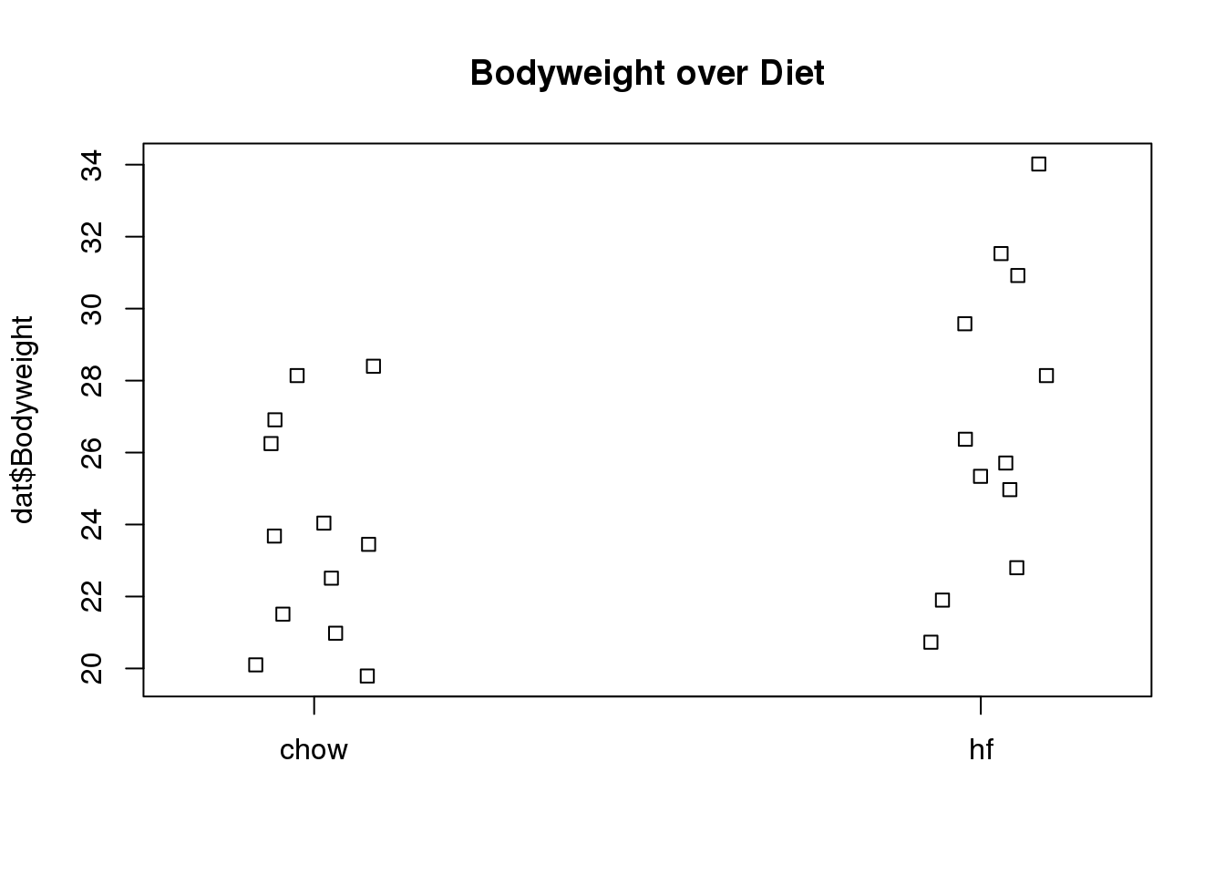
(#fig:bodyweight_by_diet_stripchart)Mice bodyweights stratified by diet.
We can see that the high fat diet group appears to have higher weights on average, although there is overlap between the two samples.
For demonstration purposes, we will build the design matrix \(\mathbf{X}\) using the formula ~ Diet. The group with the 1’s in the second column is determined by the level of Diet which comes second; that is, the non-reference level.
levels(dat$Diet)## [1] "chow" "hf"X <- model.matrix(~ Diet, data=dat)
head(X)## (Intercept) Diethf
## 1 1 0
## 2 1 0
## 3 1 0
## 4 1 0
## 5 1 0
## 6 1 05.2 The Mathematics Behind lm()
Before we use our shortcut for running linear models, lm, we want to review what will happen internally. Inside of lm, we will form the design matrix \(\mathbf{X}\) and calculate the \(\boldsymbol{\beta}\), which minimizes the sum of squares using the previously described formula. The formula for this solution is:
\[ \hat{\boldsymbol{\beta}} = (\mathbf{X}^\top \mathbf{X})^{-1} \mathbf{X}^\top \mathbf{Y} \]
We can calculate this in R using our matrix multiplication operator %*%, the inverse function solve, and the transpose function t.
Y <- dat$Bodyweight
X <- model.matrix(~ Diet, data=dat)
solve(t(X) %*% X) %*% t(X) %*% Y
## [,1]
## (Intercept) 23.813
## Diethf 3.021These coefficients are the average of the control group and the difference of the averages:
s <- split(dat$Bodyweight, dat$Diet)
mean(s[["chow"]])
## [1] 23.81mean(s[["hf"]]) - mean(s[["chow"]])## [1] 3.021Finally, we use our shortcut, lm, to run the linear model:
fit <- lm(Bodyweight ~ Diet, data=dat)
summary(fit)
##
## Call:
## lm(formula = Bodyweight ~ Diet, data = dat)
##
## Residuals:
## Min 1Q Median 3Q Max
## -6.104 -2.436 -0.414 2.834 7.186
##
## Coefficients:
## Estimate Std. Error t value Pr(>|t|)
## (Intercept) 23.81 1.04 22.91 <2e-16 ***
## Diethf 3.02 1.47 2.06 0.052 .
## ---
## Signif. codes:
## 0 '***' 0.001 '**' 0.01 '*' 0.05 '.' 0.1 ' ' 1
##
## Residual standard error: 3.6 on 22 degrees of freedom
## Multiple R-squared: 0.161, Adjusted R-squared: 0.123
## F-statistic: 4.22 on 1 and 22 DF, p-value: 0.0519(coefs <- coef(fit))## (Intercept) Diethf
## 23.813 3.0215.2.0.1 Examining the coefficients
The following plot provides a visualization of the meaning of the coefficients with colored arrows (code not shown):
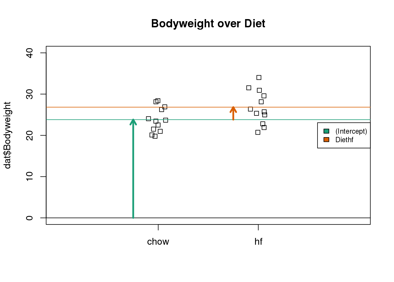
(#fig:parameter_estimate_illustration)Estimated linear model coefficients for bodyweight data illustrated with arrows.
To make a connection with material presented earlier, this simple linear model is actually giving us the same result (the t-statistic and p-value) for the difference as a specific kind of t-test. This is the t-test between two groups with the assumption that the population standard deviation is the same for both groups. This was encoded into our linear model when we assumed that the errors \(\boldsymbol{\varepsilon}\) were all equally distributed.
Although in this case the linear model is equivalent to a t-test, we will soon explore more complicated designs, where the linear model is a useful extension. Below we demonstrate that one does in fact get the exact same results:
Our lm estimates were:
summary(fit)$coefficients## Estimate Std. Error t value Pr(>|t|)
## (Intercept) 23.813 1.039 22.912 7.642e-17
## Diethf 3.021 1.470 2.055 5.192e-02And the t-statistic is the same:
ttest <- t.test(s[["hf"]], s[["chow"]], var.equal=TRUE)
summary(fit)$coefficients[2,3]
## [1] 2.055ttest$statistic## t
## 2.0555.3 Standard Errors
We have shown how to find the least squares estimates with matrix algebra. These estimates are random variables since they are linear combinations of the data. For these estimates to be useful, we also need to compute their standard errors. Linear algebra provides a powerful approach for this task. We provide several examples.
5.3.0.1 Falling object
It is useful to think about where randomness comes from. In our falling object example, randomness was introduced through measurement errors. Each time we rerun the experiment, a new set of measurement errors will be made. This implies that our data will change randomly, which in turn suggests that our estimates will change randomly. For instance, our estimate of the gravitational constant will change every time we perform the experiment. The constant is fixed, but our estimates are not. To see this we can run a Monte Carlo simulation. Specifically, we will generate the data repeatedly and each time compute the estimate for the quadratic term.
set.seed(1)
B <- 10000
h0 <- 56.67
v0 <- 0
g <- 9.8 ##meters per second

n <- 25
tt <- seq(0,3.4,len=n) ##time in secs, t is a base function
X <-cbind(1,tt,tt^2)
##create X'X^-1 X'
A <- solve(crossprod(X)) %*% t(X)
betahat<-replicate(B,{
  y <- h0 + v0*tt  - 0.5*g*tt^2 + rnorm(n,sd=1)
  betahats <- A%*%y
  return(betahats[3])
})
head(betahat)
## [1] -5.039 -4.894 -5.144 -5.221 -5.063 -4.778As expected, the estimate is different every time. This is because \(\hat{\beta}\) is a random variable. It therefore has a distribution:
library(rafalib)
mypar(1,2)
hist(betahat)
qqnorm(betahat)
qqline(betahat)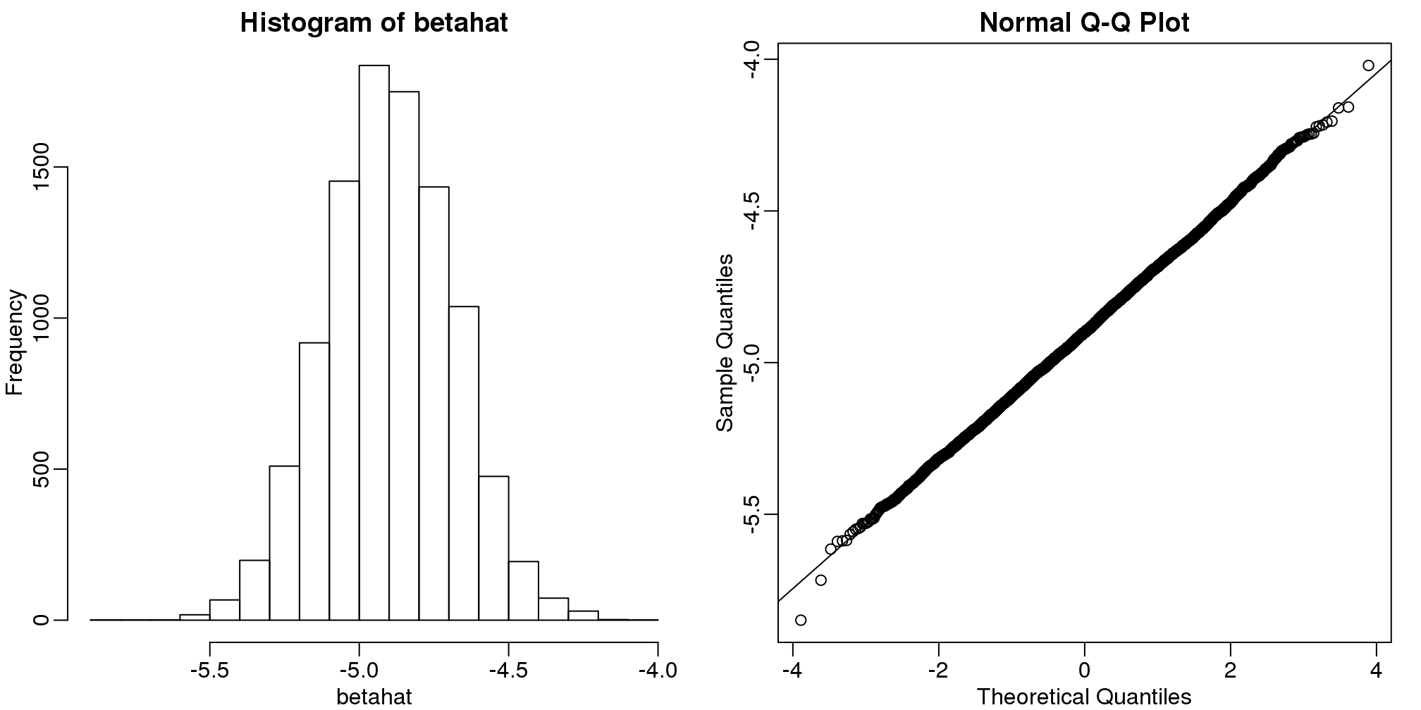
(#fig:regression_estimates_normally_distributed)Distribution of estimated regression coefficients obtained from Monte Carlo simulated falling object data. The left is a histogram and on the right we have a qq-plot against normal theoretical quantiles.
Since \(\hat{\beta}\) is a linear combination of the data which we made normal in our simulation, it is also normal as seen in the qq-plot above. Also, the mean of the distribution is the true parameter \(-0.5g\), as confirmed by the Monte Carlo simulation performed above.
round(mean(betahat),1)## [1] -4.9But we will not observe this exact value when we estimate because the standard error of our estimate is approximately:
sd(betahat) ## [1] 0.213Here we will show how we can compute the standard error without a Monte Carlo simulation. Since in practice we do not know exactly how the errors are generated, we can’t use the Monte Carlo approach.
5.3.0.2 Father and son heights
In the father and son height examples, we have randomness because we have a random sample of father and son pairs. For the sake of illustration, let’s assume that this is the entire population:
data(father.son,package="UsingR")
x <- father.son$fheight
y <- father.son$sheight
n <- length(y)
Now let’s run a Monte Carlo simulation in which we take a sample size of 50 over and over again.
N <- 50
B <-1000
betahat <- replicate(B,{
  index <- sample(n,N)
  sampledat <- father.son[index,]
  x <- sampledat$fheight
  y <- sampledat$sheight
  lm(y~x)$coef
  })
betahat <- t(betahat) #have estimates in two columns
By making qq-plots, we see that our estimates are approximately normal random variables:
mypar(1,2)
qqnorm(betahat[,1])
qqline(betahat[,1])
qqnorm(betahat[,2])
qqline(betahat[,2])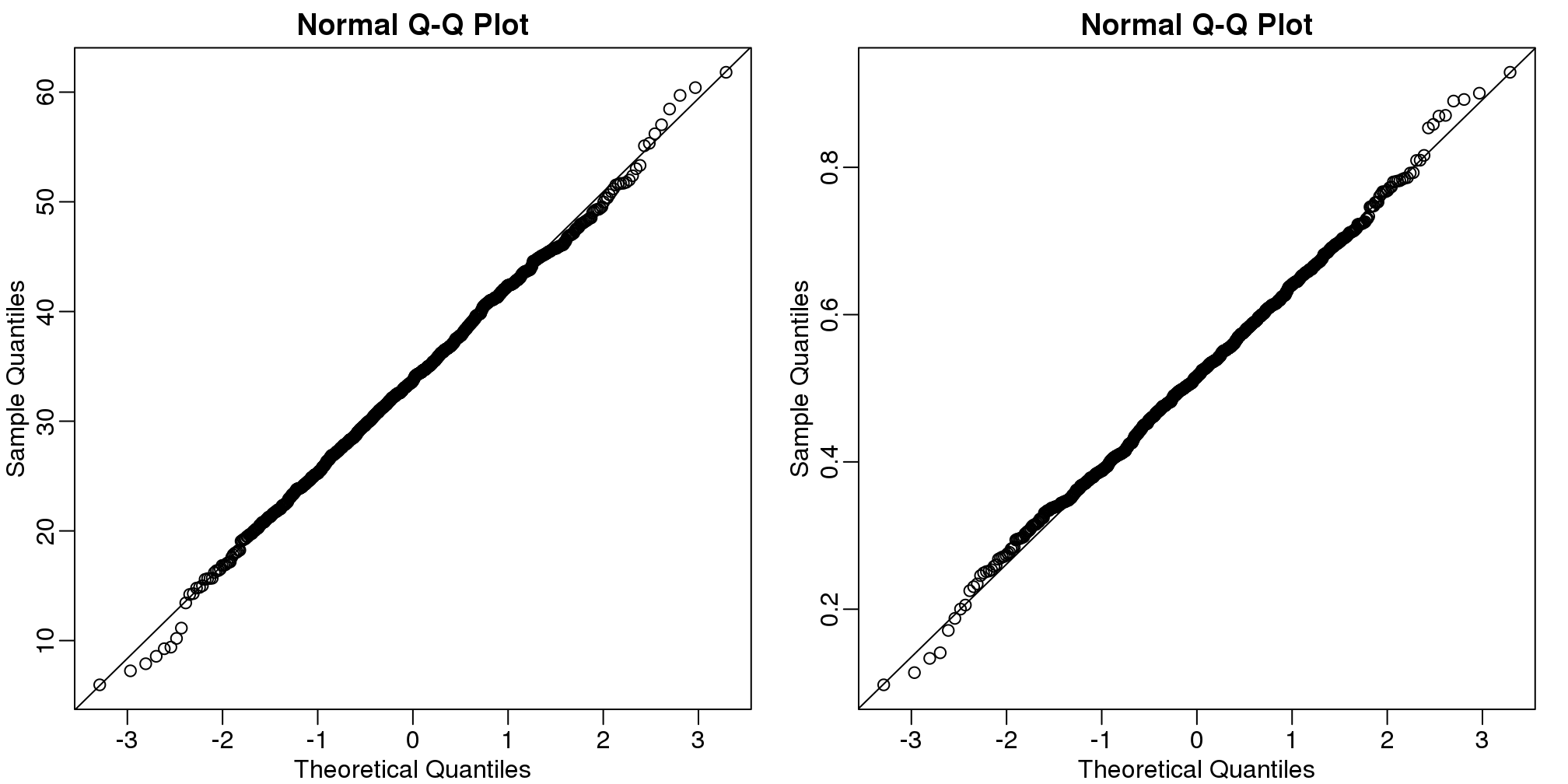
(#fig:regression_estimates_normally_distributed2)Distribution of estimated regression coefficients obtained from Monte Carlo simulated father-son height data. The left is a histogram and on the right we have a qq-plot against normal theoretical quantiles.
We also see that the correlation of our estimates is negative:
cor(betahat[,1],betahat[,2])## [1] -0.9992When we compute linear combinations of our estimates, we will need to know this information to correctly calculate the standard error of these linear combinations.
In the next section, we will describe the variance-covariance matrix. The covariance of two random variables is defined as follows:
mean( (betahat[,1]-mean(betahat[,1] ))* (betahat[,2]-mean(betahat[,2])))## [1] -1.035The covariance is the correlation multiplied by the standard deviations of each random variable:
\[\mbox{Corr}(X,Y) = \frac{\mbox{Cov}(X,Y)}{\sigma_X \sigma_Y}\]
Other than that, this quantity does not have a useful interpretation in practice. However, as we will see, it is a very useful quantity for mathematical derivations. In the next sections, we show useful matrix algebra calculations that can be used to estimate standard errors of linear model estimates.
5.3.0.3 Variance-covariance matrix (Advanced)
As a first step we need to define the variance-covariance matrix, \(\boldsymbol{\Sigma}\). For a vector of random variables, \(\mathbf{Y}\), we define \(\boldsymbol{\Sigma}\) as the matrix with the \(i,j\) entry:
\[ \Sigma_{i,j} \equiv \mbox{Cov}(Y_i, Y_j) \]
The covariance is equal to the variance if \(i = j\) and equal to 0 if the variables are independent. In the kinds of vectors considered up to now, for example, a vector \(\mathbf{Y}\) of individual observations \(Y_i\) sampled from a population, we have assumed independence of each observation and assumed the \(Y_i\) all have the same variance \(\sigma^2\), so the variance-covariance matrix has had only two kinds of elements:
\[ \mbox{Cov}(Y_i, Y_i) = \mbox{var}(Y_i) = \sigma^2\]
\[ \mbox{Cov}(Y_i, Y_j) = 0, \mbox{ for } i \neq j\]
which implies that \(\boldsymbol{\Sigma} = \sigma^2 \mathbf{I}\) with \(\mathbf{I}\), the identity matrix.
Later, we will see a case, specifically the estimate coefficients of a linear model, \(\hat{\boldsymbol{\beta}}\), that has non-zero entries in the off diagonal elements of \(\boldsymbol{\Sigma}\). Furthermore, the diagonal elements will not be equal to a single value \(\sigma^2\).
5.3.0.4 Variance of a linear combination
A useful result provided by linear algebra is that the variance covariance-matrix of a linear combination \(\mathbf{AY}\) of \(\mathbf{Y}\) can be computed as follows:
\[ \mbox{var}(\mathbf{AY}) = \mathbf{A}\mbox{var}(\mathbf{Y}) \mathbf{A}^\top \]
For example, if \(Y_1\) and \(Y_2\) are independent both with variance \(\sigma^2\) then:
\[\mbox{var}\{Y_1+Y_2\} = \mbox{var}\left\{ \begin{pmatrix}1&1\end{pmatrix}\begin{pmatrix} Y_1\\Y_2\\ \end{pmatrix}\right\}\]
\[ =\begin{pmatrix}1&1\end{pmatrix} \sigma^2 \mathbf{I}\begin{pmatrix} 1\\1\\ \end{pmatrix}=2\sigma^2\]
as we expect. We use this result to obtain the standard errors of the LSE (least squares estimate).
5.3.0.5 LSE standard errors (Advanced)
Note that \(\boldsymbol{\hat{\beta}}\) is a linear combination of \(\mathbf{Y}\): \(\mathbf{AY}\) with \(\mathbf{A}=\mathbf{(X^\top X)^{-1}X}^\top\), so we can use the equation above to derive the variance of our estimates:
\[\mbox{var}(\boldsymbol{\hat{\beta}}) = \mbox{var}( \mathbf{(X^\top X)^{-1}X^\top Y} ) = \]
\[\mathbf{(X^\top X)^{-1} X^\top} \mbox{var}(Y) (\mathbf{(X^\top X)^{-1} X^\top})^\top = \]
\[\mathbf{(X^\top X)^{-1} X^\top} \sigma^2 \mathbf{I} (\mathbf{(X^\top X)^{-1} X^\top})^\top = \]
\[\sigma^2 \mathbf{(X^\top X)^{-1} X^\top}\mathbf{X} \mathbf{(X^\top X)^{-1}} = \]
\[\sigma^2\mathbf{(X^\top X)^{-1}}\]
The diagonal of the square root of this matrix contains the standard error of our estimates.
5.3.0.6 Estimating \(\sigma^2\)
To obtain an actual estimate in practice from the formulas above, we need to estimate \(\sigma^2\). Previously we estimated the standard errors from the sample. However, the sample standard deviation of \(Y\) is not \(\sigma\) because \(Y\) also includes variability introduced by the deterministic part of the model: \(\mathbf{X}\boldsymbol{\beta}\). The approach we take is to use the residuals.
We form the residuals like this:
\[ \mathbf{r}\equiv\boldsymbol{\hat{\varepsilon}} = \mathbf{Y}-\mathbf{X}\boldsymbol{\hat{\beta}}\]
Both \(\mathbf{r}\) and \(\boldsymbol{\hat{\varepsilon}}\) notations are used to denote residuals.
Then we use these to estimate, in a similar way, to what we do in the univariate case:
\[ s^2 \equiv \hat{\sigma}^2 = \frac{1}{N-p}\mathbf{r}^\top\mathbf{r} = \frac{1}{N-p}\sum_{i=1}^N r_i^2\]
Here \(N\) is the sample size and \(p\) is the number of columns in \(\mathbf{X}\) or number of parameters (including the intercept term \(\beta_0\)). The reason we divide by \(N-p\) is because mathematical theory tells us that this will give us a better (unbiased) estimate.
Let’s try this in R and see if we obtain the same values as we did with the Monte Carlo simulation above:
n <- nrow(father.son)
N <- 50
index <- sample(n,N)
sampledat <- father.son[index,]
x <- sampledat$fheight
y <- sampledat$sheight
X <- model.matrix(~x)

N <- nrow(X)
p <- ncol(X)

XtXinv <- solve(crossprod(X))

resid <- y - X %*% XtXinv %*% crossprod(X,y)

s <- sqrt( sum(resid^2)/(N-p))
ses <- sqrt(diag(XtXinv))*s
Let’s compare to what lm provides:
summary(lm(y~x))$coef[,2]## (Intercept) x
## 8.3900 0.1241ses## (Intercept) x
## 8.3900 0.1241They are identical because they are doing the same thing. Also, note that we approximate the Monte Carlo results:
apply(betahat,2,sd)## (Intercept) x
## 8.3818 0.12375.3.0.7 Linear combination of estimates
Frequently, we want to compute the standard deviation of a linear combination of estimates such as \(\hat{\beta}_2 - \hat{\beta}_1\). This is a linear combination of \(\hat{\boldsymbol{\beta}}\):
\[\hat{\beta}_2 - \hat{\beta}_1 = \begin{pmatrix}0&-1&1&0&\dots&0\end{pmatrix} \begin{pmatrix} \hat{\beta}_0\\ \hat{\beta}_1 \\ \hat{\beta}_2 \\ \vdots\\ \hat{\beta}_p \end{pmatrix}\]
Using the above, we know how to compute the variance covariance matrix of \(\hat{\boldsymbol{\beta}}\).
5.3.0.8 CLT and t-distribution
We have shown how we can obtain standard errors for our estimates. However, as we learned in the first chapter, to perform inference we need to know the distribution of these random variables. The reason we went through the effort to compute the standard errors is because the CLT applies in linear models. If \(N\) is large enough, then the LSE will be normally distributed with mean \(\boldsymbol{\beta}\) and standard errors as described. For small samples, if the \(\varepsilon\) are normally distributed, then the \(\hat{\beta}-\beta\) follow a t-distribution. We do not derive this result here, but the results are extremely useful since it is how we construct p-values and confidence intervals in the context of linear models.
5.3.0.9 Code versus math
The standard approach to writing linear models either assume the values in \(\mathbf{X}\) are fixed or that we are conditioning on them. Thus \(\mathbf{X} \boldsymbol{\beta}\) has no variance as the \(\mathbf{X}\) is considered fixed. This is why we write \(\mbox{var}(Y_i) = \mbox{var}(\varepsilon_i)=\sigma^2\). This can cause confusion in practice because if you, for example, compute the following:
x =  father.son$fheight
beta =  c(34,0.5)
var(beta[1]+beta[2]*x)
## [1] 1.884it is nowhere near 0. This is an example in which we have to be careful in distinguishing code from math. The function var is simply computing the variance of the list we feed it, while the mathematical definition of variance is considering only quantities that are random variables. In the R code above, x is not fixed at all: we are letting it vary, but when we write \(\mbox{var}(Y_i) = \sigma^2\) we are imposing, mathematically, x to be fixed. Similarly, if we use R to compute the variance of \(Y\) in our object dropping example, we obtain something very different than \(\sigma^2=1\) (the known variance):
n <- length(tt)
y <- h0 + v0*tt  - 0.5*g*tt^2 + rnorm(n,sd=1)
var(y)
## [1] 329.5Again, this is because we are not fixing tt.
5.4 Interactions and Contrasts
As a running example to learn about more complex linear models, we will be using a dataset which compares the different frictional coefficients on the different legs of a spider. Specifically, we will be determining whether more friction comes from a pushing or pulling motion of the leg. The original paper from which the data was provided is:
Jonas O. Wolff & Stanislav N. Gorb, Radial arrangement of Janus-like setae permits friction control in spiders, Scientific Reports, 22 January 2013.
The abstract of the paper says,
The hunting spider Cupiennius salei (Arachnida, Ctenidae) possesses hairy attachment pads (claw tufts) at its distal legs, consisting of directional branched setae… Friction of claw tufts on smooth glass was measured to reveal the functional effect of seta arrangement within the pad.
Figure 1 includes some pretty cool electron microscope images of the tufts. We are interested in the comparisons in Figure 4, where the pulling and pushing motions are compared for different leg pairs (for a diagram of pushing and pulling see the top of Figure 3).
We include the data in our dagdata package and can download it from here.
spider <- read.csv("spider_wolff_gorb_2013.csv", skip=1)5.4.0.1 Initial visual inspection of the data
Each measurement comes from one of our legs while it is either pushing or pulling. So we have two variables:
table(spider$leg,spider$type)##
## pull push
## L1 34 34
## L2 15 15
## L3 52 52
## L4 40 40We can make a boxplot summarizing the measurements for each of the eight pairs. This is similar to Figure 4 of the original paper:
boxplot(spider$friction ~ spider$type * spider$leg,
        col=c("grey90","grey40"), las=2,
        main="Comparison of friction coefficients of different leg pairs")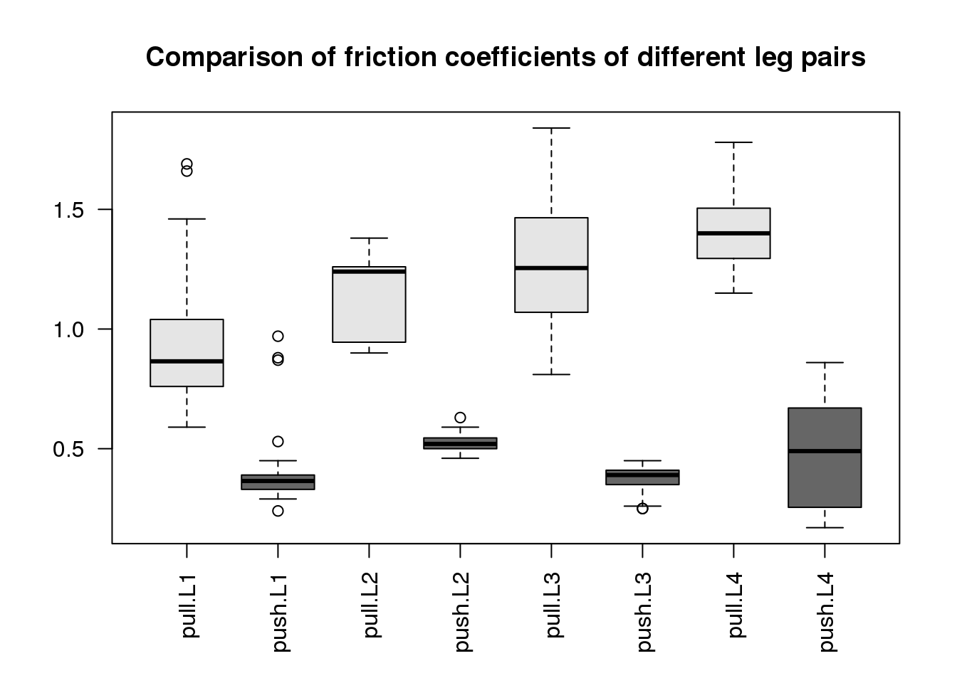
(#fig:spide_data)Comparison of friction coefficients of spiders’ different leg pairs. The friction coefficient is calculated as the ratio of two forces (see paper Methods) so it is unitless.
What we can immediately see are two trends:
- The pulling motion has higher friction than the pushing motion.
- The leg pairs to the back of the spider (L4 being the last) have higher pulling friction.
Another thing to notice is that the groups have different spread around their average, what we call within-group variance. This is somewhat of a problem for the kinds of linear models we will explore below, since we will be assuming that around the population average values, the errors \(\varepsilon_i\) are distributed identically, meaning the same variance within each group. The consequence of ignoring the different variances for the different groups is that comparisons between those groups with small variances will be overly “conservative” (because the overall estimate of variance is larger than an estimate for just these groups), and comparisons between those groups with large variances will be overly confident. If the spread is related to the range of friction, such that groups with large friction values also have larger spread, a possibility is to transform the data with a function such as the log or sqrt. This looks like it could be useful here, since three of the four push groups (L1, L2, L3) have the smallest friction values and also the smallest spread.
Some alternative tests for comparing groups without transforming the values first include: t-tests without the equal variance assumption using a “Welch” or “Satterthwaite approximation”, or the Wilcoxon rank sum test mentioned previously. However here, for simplicity of illustration, we will fit a model that assumes equal variance and shows the different kinds of linear model designs using this dataset, setting aside the issue of different within-group variances.
5.4.0.2 A linear model with one variable
To remind ourselves how the simple two-group linear model looks, we will subset the data to include only the L1 leg pair, and run lm:
spider.sub <- spider[spider$leg == "L1",]
fit <- lm(friction ~ type, data=spider.sub)
summary(fit)
##
## Call:
## lm(formula = friction ~ type, data = spider.sub)
##
## Residuals:
## Min 1Q Median 3Q Max
## -0.3315 -0.1074 -0.0494 -0.0015 0.7685
##
## Coefficients:
## Estimate Std. Error t value Pr(>|t|)
## (Intercept) 0.9215 0.0383 24.1 < 2e-16 ***
## typepush -0.5141 0.0541 -9.5 5.7e-14 ***
## ---
## Signif. codes:
## 0 '***' 0.001 '**' 0.01 '*' 0.05 '.' 0.1 ' ' 1
##
## Residual standard error: 0.223 on 66 degrees of freedom
## Multiple R-squared: 0.578, Adjusted R-squared: 0.571
## F-statistic: 90.2 on 1 and 66 DF, p-value: 5.7e-14(coefs <- coef(fit))## (Intercept) typepush
## 0.9215 -0.5141These two estimated coefficients are the mean of the pull observations (the first estimated coefficient) and the difference between the means of the two groups (the second coefficient). We can show this with R code:
s <- split(spider.sub$friction, spider.sub$type)
mean(s[["pull"]])
## [1] 0.9215mean(s[["push"]]) - mean(s[["pull"]])## [1] -0.5141We can form the design matrix, which was used inside lm:
X <- model.matrix(~ type, data=spider.sub)
colnames(X)
## [1] "(Intercept)" "typepush"head(X)## (Intercept) typepush
## 1 1 0
## 2 1 0
## 3 1 0
## 4 1 0
## 5 1 0
## 6 1 0tail(X)## (Intercept) typepush
## 63 1 1
## 64 1 1
## 65 1 1
## 66 1 1
## 67 1 1
## 68 1 1Now we’ll make a plot of the \(\mathbf{X}\) matrix by putting a black block for the 1’s and a white block for the 0’s. This plot will be more interesting for the linear models later on in this script. Along the y-axis is the sample number (the row number of the data) and along the x-axis is the column of the design matrix \(\mathbf{X}\). If you have installed the rafalib library, you can make this plot with the imagemat function:
library(rafalib)
imagemat(X, main="Model matrix for linear model with one variable")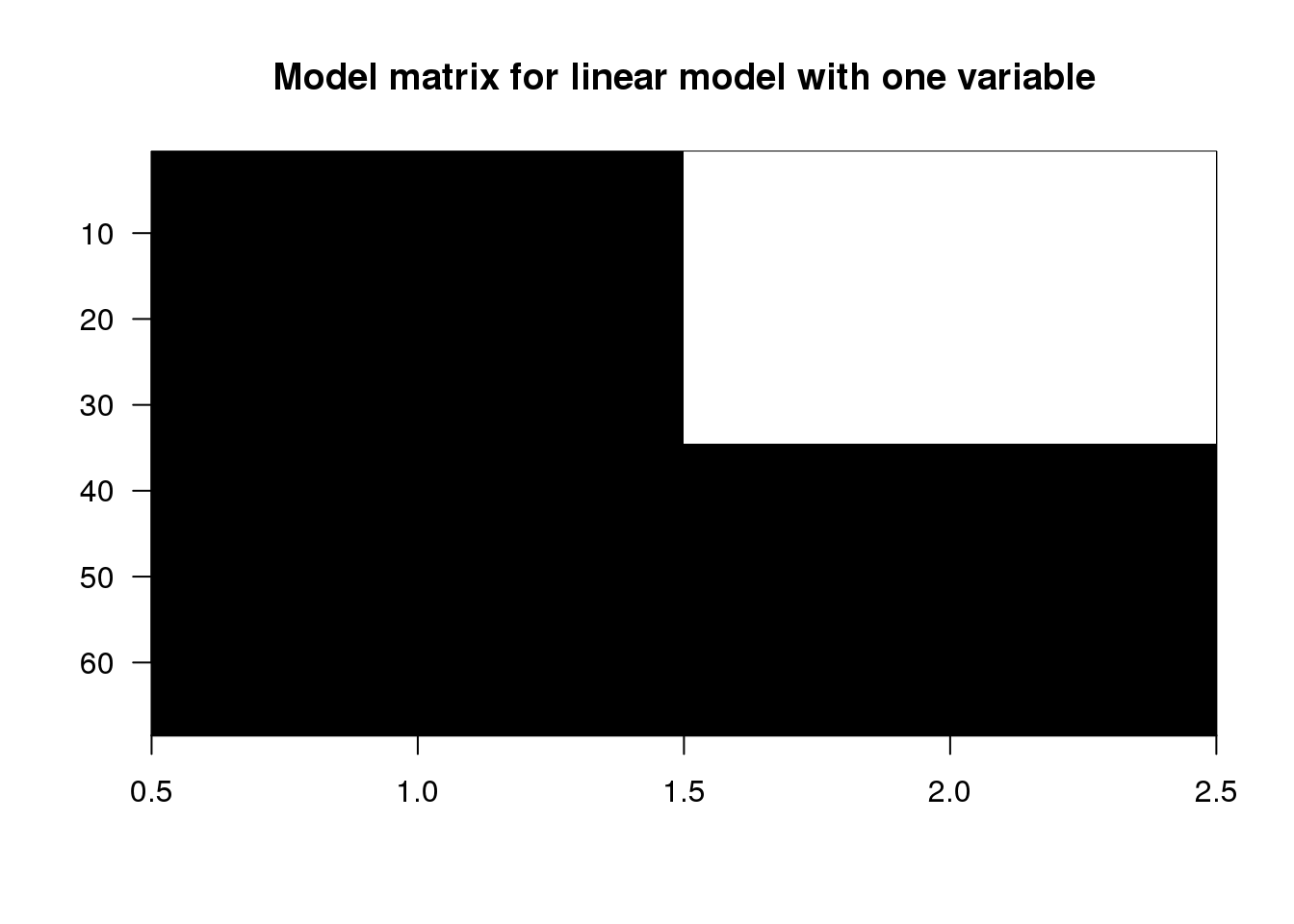
(#fig:model_matrix_image)Model matrix for linear model with one variable.
5.4.0.3 Examining the estimated coefficients
Now we show the coefficient estimates from the linear model in a diagram with arrows (code not shown).
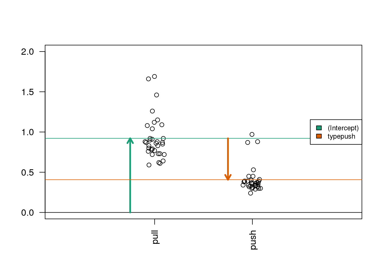
(#fig:spider_main_coef)Diagram of the estimated coefficients in the linear model. The green arrow indicates the Intercept term, which goes from zero to the mean of the reference group (here the ‘pull’ samples). The orange arrow indicates the difference between the push group and the pull group, which is negative in this example. The circles show the individual samples, jittered horizontally to avoid overplotting.
5.4.0.4 A linear model with two variables
Now we’ll continue and examine the full dataset, including the observations from all leg pairs. In order to model both the leg pair differences (L1, L2, L3, L4) and the push vs. pull difference, we need to include both terms in the R formula. Let’s see what kind of design matrix will be formed with two variables in the formula:
X <- model.matrix(~ type + leg, data=spider)
colnames(X)
## [1] "(Intercept)" "typepush" "legL2"
## [4] "legL3" "legL4"head(X)## (Intercept) typepush legL2 legL3 legL4
## 1 1 0 0 0 0
## 2 1 0 0 0 0
## 3 1 0 0 0 0
## 4 1 0 0 0 0
## 5 1 0 0 0 0
## 6 1 0 0 0 0imagemat(X, main="Model matrix for linear model with two factors")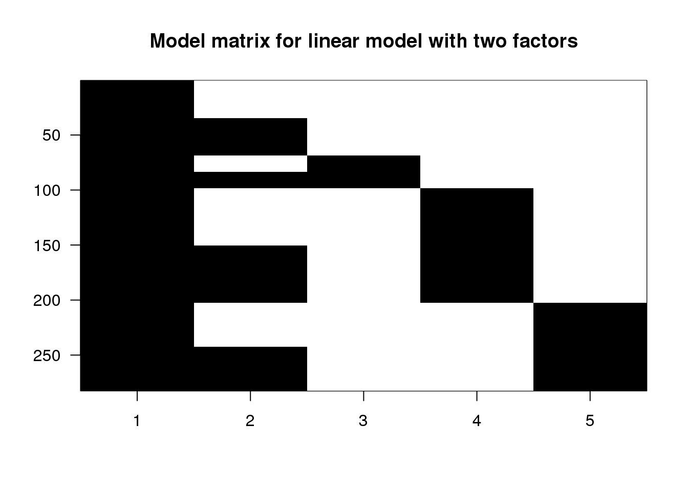
(#fig:model_matrix_image2)Image of the model matrix for a formula with type + leg
The first column is the intercept, and so it has 1’s for all samples. The second column has 1’s for the push samples, and we can see that there are four groups of them. Finally, the third, fourth and fifth columns have 1’s for the L2, L3 and L4 samples. The L1 samples do not have a column, because L1 is the reference level for leg. Similarly, there is no pull column, because pull is the reference level for the type variable.
To estimate coefficients for this model, we use lm with the formula ~ type + leg. We’ll save the linear model to fitTL standing for a fit with Type and Leg.
fitTL <- lm(friction ~ type + leg, data=spider)
summary(fitTL)
##
## Call:
## lm(formula = friction ~ type + leg, data = spider)
##
## Residuals:
## Min 1Q Median 3Q Max
## -0.4639 -0.1344 -0.0053 0.1055 0.6951
##
## Coefficients:
## Estimate Std. Error t value Pr(>|t|)
## (Intercept) 1.0539 0.0282 37.43 < 2e-16 ***
## typepush -0.7790 0.0248 -31.38 < 2e-16 ***
## legL2 0.1719 0.0457 3.76 2e-04 ***
## legL3 0.1605 0.0325 4.94 1.4e-06 ***
## legL4 0.2813 0.0344 8.18 1.0e-14 ***
## ---
## Signif. codes:
## 0 '***' 0.001 '**' 0.01 '*' 0.05 '.' 0.1 ' ' 1
##
## Residual standard error: 0.208 on 277 degrees of freedom
## Multiple R-squared: 0.792, Adjusted R-squared: 0.789
## F-statistic: 263 on 4 and 277 DF, p-value: <2e-16(coefs <- coef(fitTL))## (Intercept) typepush legL2 legL3
## 1.0539 -0.7790 0.1719 0.1605
## legL4
## 0.2813R uses the name coefficient to denote the component containing the least squares estimates. It is important to remember that the coefficients are parameters that we do not observe, but only estimate.
5.4.0.5 Mathematical representation
The model we are fitting above can be written as
\[ Y_i = \beta_0 + \beta_1 x_{i,1} + \beta_2 x_{i,2} + \beta_3 x_{i,3} + \beta_4 x_{i,4} + \varepsilon_i, i=1,\dots,N \]
with the \(x\) all indicator variables denoting push or pull and which leg. For example, a push on leg 3 will have \(x_{i,1}\) and \(x_{i,3}\) equal to 1 and the rest would be 0. Throughout this section we will refer to the \(\beta\) s with the effects they represent. For example we call \(\beta_0\) the intercept, \(\beta_1\) the pull effect, \(\beta_2\) the L2 effect, etc. We do not observe the coefficients, e.g. \(\beta_1\), directly, but estimate them with, e.g. \(\hat{\beta}_4\).
We can now form the matrix \(\mathbf{X}\) depicted above and obtain the least square estimates with:
\[ \hat{\boldsymbol{\beta}} = (\mathbf{X}^\top \mathbf{X})^{-1} \mathbf{X}^\top \mathbf{Y} \]
Y <- spider$friction
X <- model.matrix(~ type + leg, data=spider)
beta.hat <- solve(t(X) %*% X) %*% t(X) %*% Y
t(beta.hat)
## (Intercept) typepush legL2 legL3 legL4
## [1,] 1.054 -0.779 0.1719 0.1605 0.2813coefs## (Intercept) typepush legL2 legL3
## 1.0539 -0.7790 0.1719 0.1605
## legL4
## 0.2813We can see that these values agree with the output of lm.
5.4.0.6 Examining the estimated coefficients
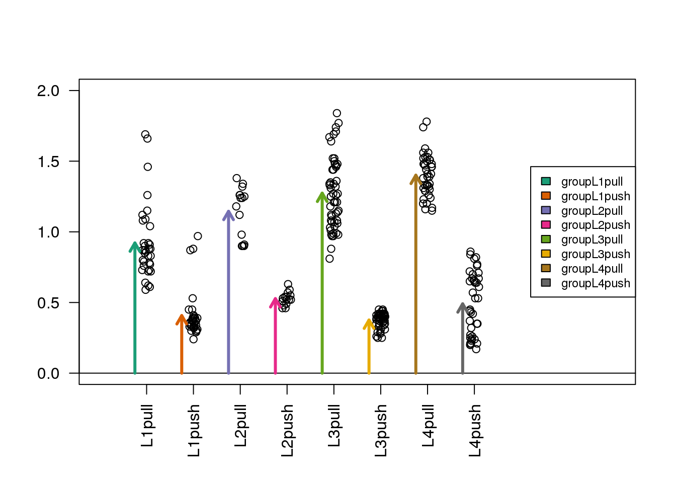
We can make the same plot as before, with arrows for each of the estimated coefficients in the model (code not shown).
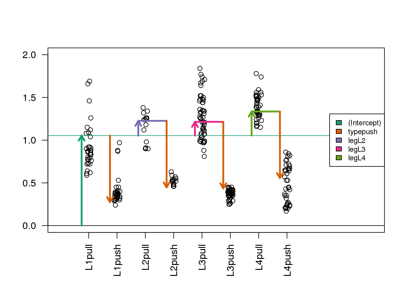
(#fig:spider_interactions)Diagram of the estimated coefficients in the linear model. As before, the teal-green arrow represents the Intercept, which fits the mean of the reference group (here, the pull samples for leg L1). The purple, pink, and yellow-green arrows represent differences between the three other leg groups and L1. The orange arrow represents the difference between the push and pull samples for all groups.
In this case, the fitted means for each group, derived from the fitted coefficients, do not line up with those we obtain from simply taking the average from each of the eight possible groups. The reason is that our model uses five coefficients, instead of eight. We are assuming that the effects are additive. However, as we demonstrate in more detail below, this particular dataset is better described with a model including interactions.
s <- split(spider$friction, spider$group)
mean(s[["L1pull"]])
## [1] 0.9215coefs[1]## (Intercept)
## 1.054mean(s[["L1push"]])## [1] 0.4074coefs[1] + coefs[2]## (Intercept)
## 0.2749Here we can demonstrate that the push vs. pull estimated coefficient, coefs[2], is a weighted average of the difference of the means for each group. Furthermore, the weighting is determined by the sample size of each group. The math works out simply here because the sample size is equal for the push and pull subgroups within each leg pair. If the sample sizes were not equal for push and pull within each leg pair, the weighting is more complicated but uniquely determined by a formula involving the sample size of each subgroup, the total sample size, and the number of coefficients. This can be worked out from \((\mathbf{X}^\top \mathbf{X})^{-1} \mathbf{X}^\top\).
means <- sapply(s, mean)
##the sample size of push or pull groups for each leg pair
ns <- sapply(s, length)[c(1,3,5,7)]
(w <- ns/sum(ns))
## L1pull L2pull L3pull L4pull
## 0.2411 0.1064 0.3688 0.2837sum(w * (means[c(2,4,6,8)] - means[c(1,3,5,7)]))## [1] -0.779coefs[2]## typepush
## -0.7795.4.0.7 Contrasting coefficients
Sometimes, the comparison we are interested in is represented directly by a single coefficient in the model, such as the push vs. pull difference, which was coefs[2] above. However, sometimes, we want to make a comparison which is not a single coefficient, but a combination of coefficients, which is called a contrast. To introduce the concept of contrasts, first consider the comparisons which we can read off from the linear model summary:
coefs## (Intercept) typepush legL2 legL3
## 1.0539 -0.7790 0.1719 0.1605
## legL4
## 0.2813Here we have the intercept estimate, the push vs. pull estimated effect across all leg pairs, and the estimates for the L2 vs. L1 effect, the L3 vs. L1 effect, and the L4 vs. L1 effect. What if we want to compare two groups and one of those groups is not L1? The solution to this question is to use contrasts.
A contrast is a combination of estimated coefficient: \(\mathbf{c^\top} \hat{\boldsymbol{\beta}}\), where \(\mathbf{c}\) is a column vector with as many rows as the number of coefficients in the linear model. If \(\mathbf{c}\) has a 0 for one or more of its rows, then the corresponding estimated coefficients in \(\hat{\boldsymbol{\beta}}\) are not involved in the contrast.
If we want to compare leg pairs L3 and L2, this is equivalent to contrasting two coefficients from the linear model because, in this contrast, the comparison to the reference level L1 cancels out:
\[ (\mbox{L3} - \mbox{L1}) - (\mbox{L2} - \mbox{L1}) = \mbox{L3} - \mbox{L2 }\]
An easy way to make these contrasts of two groups is to use the contrast function from the contrast package. We just need to specify which groups we want to compare. We have to pick one of pull or push types, although the answer will not differ, as we will see below.
library(contrast) #Available from CRAN
L3vsL2 <- contrast(fitTL,list(leg="L3",type="pull"),list(leg="L2",type="pull"))
L3vsL2
## lm model parameter contrast
##
## Contrast S.E. Lower Upper t df Pr(>|t|)
## -0.01143 0.0432 -0.09647 0.07361 -0.26 277 0.7915The first column Contrast gives the L3 vs. L2 estimate from the model we fit above.
We can show that the least squares estimates of a linear combination of coefficients is the same linear combination of the estimates. Therefore, the effect size estimate is just the difference between two estimated coefficients. The contrast vector used by contrast is stored as a variable called X within the resulting object (not to be confused with our original \(\mathbf{X}\), the design matrix).
coefs[4] - coefs[3]## legL3
## -0.01143(cT <- L3vsL2$X)## (Intercept) typepush legL2 legL3 legL4
## 1 0 0 -1 1 0
## attr(,"assign")
## [1] 0 1 2 2 2
## attr(,"contrasts")
## attr(,"contrasts")$type
## [1] "contr.treatment"
##
## attr(,"contrasts")$leg
## [1] "contr.treatment"cT %*% coefs## [,1]
## 1 -0.01143What about the standard error and t-statistic? As before, the t-statistic is the estimate divided by the standard error. The standard error of the contrast estimate is formed by multiplying the contrast vector \(\mathbf{c}\) on either side of the estimated covariance matrix, \(\hat{\Sigma}\), our estimate for \(\mathrm{var}(\hat{\boldsymbol{\beta}})\):
\[ \sqrt{\mathbf{c^\top} \hat{\boldsymbol{\Sigma}} \mathbf{c}} \]
where we saw the covariance of the coefficients earlier:
\[ \boldsymbol{\Sigma} = \sigma^2 (\mathbf{X}^\top \mathbf{X})^{-1} \]
We estimate \(\sigma^2\) with the sample estimate \(\hat{\sigma}^2\) described above and obtain:
Sigma.hat <- sum(fitTL$residuals^2)/(nrow(X) - ncol(X)) * solve(t(X) %*% X)
signif(Sigma.hat, 2)
## (Intercept) typepush legL2 legL3
## (Intercept) 0.00079 -3.1e-04 -0.00064 -0.00064
## typepush -0.00031 6.2e-04 0.00000 0.00000
## legL2 -0.00064 -6.4e-20 0.00210 0.00064
## legL3 -0.00064 -6.4e-20 0.00064 0.00110
## legL4 -0.00064 -1.2e-19 0.00064 0.00064
## legL4
## (Intercept) -0.00064
## typepush 0.00000
## legL2 0.00064
## legL3 0.00064
## legL4 0.00120sqrt(cT %*% Sigma.hat %*% t(cT))## 1
## 1 0.0432L3vsL2$SE## [1] 0.0432We would have obtained the same result for a contrast of L3 and L2 had we picked type="push". The reason it does not change the contrast is because it leads to addition of the typepush effect on both sides of the difference, which cancels out:
L3vsL2.equiv <- contrast(fitTL,list(leg="L3",type="push"),list(leg="L2",type="push"))
L3vsL2.equiv$X
## (Intercept) typepush legL2 legL3 legL4
## 1 0 0 -1 1 0
## attr(,"assign")
## [1] 0 1 2 2 2
## attr(,"contrasts")
## attr(,"contrasts")$type
## [1] "contr.treatment"
##
## attr(,"contrasts")$leg
## [1] "contr.treatment"5.5 Linear Model with Interactions
In the previous linear model, we assumed that the push vs. pull effect was the same for all of the leg pairs (the same orange arrow). You can easily see that this does not capture the trends in the data that well. That is, the tips of the arrows did not line up perfectly with the group averages. For the L1 leg pair, the push vs. pull estimated coefficient was too large, and for the L3 leg pair, the push vs. pull coefficient was somewhat too small.
Interaction terms will help us overcome this problem by introducing additional coefficients to compensate for differences in the push vs. pull effect across the 4 groups. As we already have a push vs. pull term in the model, we only need to add three more terms to have the freedom to find leg-pair-specific push vs. pull differences. As we will see, interaction terms are added to the design matrix by multiplying the columns of the design matrix representing existing terms.
We can rebuild our linear model with an interaction between type and leg, by including an extra term in the formula type:leg. The : symbol adds an interaction between the two variables surrounding it. An equivalent way to specify this model is ~ type*leg, which will expand to the formula ~ type + leg + type:leg, with main effects for type, leg and an interaction term type:leg.
X <- model.matrix(~ type + leg + type:leg, data=spider)
colnames(X)
## [1] "(Intercept)" "typepush" "legL2"
## [4] "legL3" "legL4" "typepush:legL2"
## [7] "typepush:legL3" "typepush:legL4"head(X)## (Intercept) typepush legL2 legL3 legL4
## 1 1 0 0 0 0
## 2 1 0 0 0 0
## 3 1 0 0 0 0
## 4 1 0 0 0 0
## 5 1 0 0 0 0
## 6 1 0 0 0 0
## typepush:legL2 typepush:legL3 typepush:legL4
## 1 0 0 0
## 2 0 0 0
## 3 0 0 0
## 4 0 0 0
## 5 0 0 0
## 6 0 0 0imagemat(X, main="Model matrix for linear model with interactions")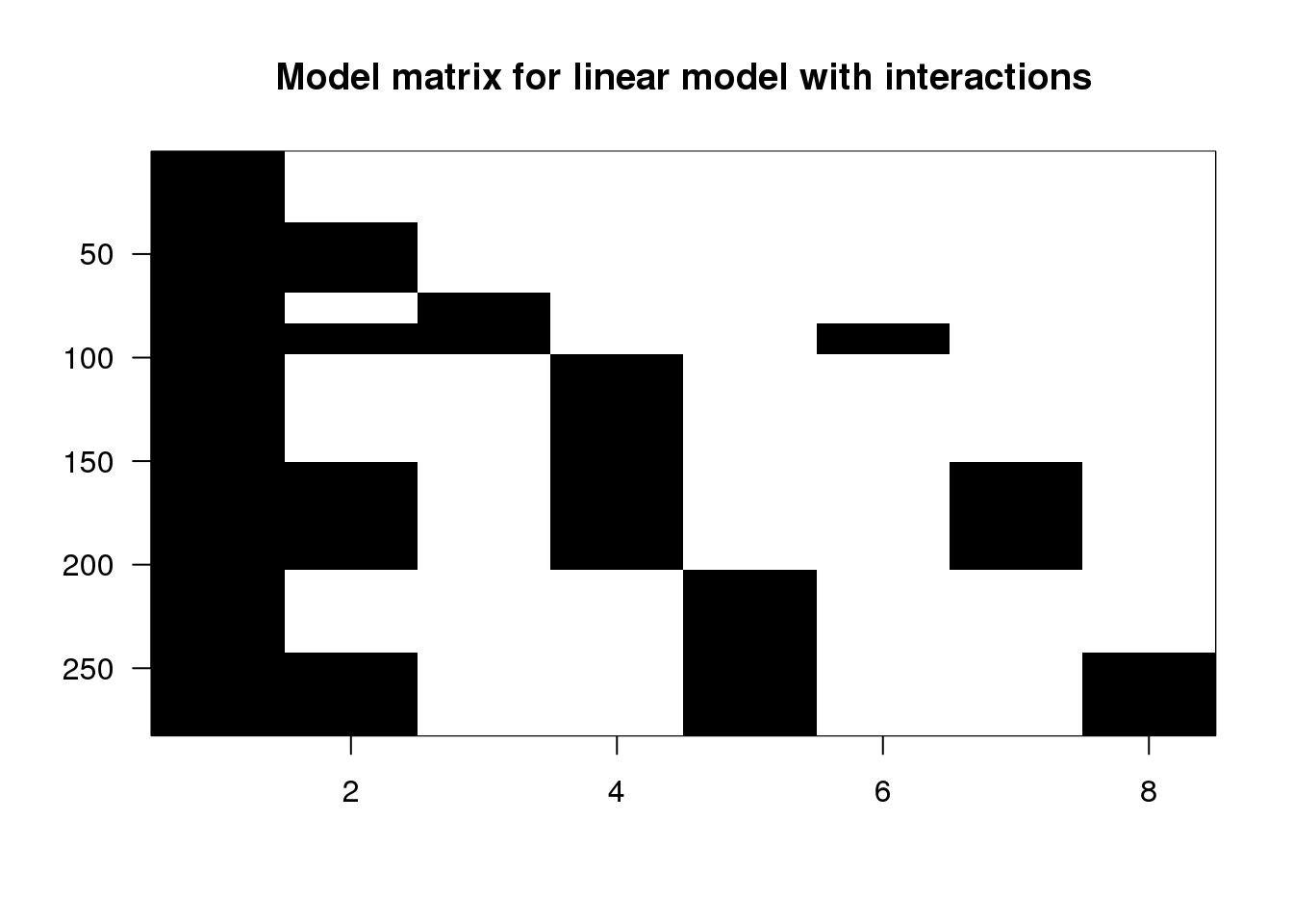
(#fig:model_matrix_with_interaction_image)Image of model matrix with interactions.
Columns 6-8 (typepush:legL2, typepush:legL3, and typepush:legL4) are the product of the 2nd column (typepush) and columns 3-5 (the three leg columns). Looking at the last column, for example, the typepush:legL4 column is adding an extra coefficient \(\beta_{\textrm{push,L4}}\) to those samples which are both push samples and leg pair L4 samples. This accounts for a possible difference when the mean of samples in the L4-push group are not at the location which would be predicted by adding the estimated intercept, the estimated push coefficient typepush, and the estimated L4 coefficient legL4.
We can run the linear model using the same code as before:
fitX <- lm(friction ~ type + leg + type:leg, data=spider)
summary(fitX)
##
## Call:
## lm(formula = friction ~ type + leg + type:leg, data = spider)
##
## Residuals:
## Min 1Q Median 3Q Max
## -0.4638 -0.1074 -0.0111 0.0785 0.7685
##
## Coefficients:
## Estimate Std. Error t value Pr(>|t|)
## (Intercept) 0.9215 0.0327 28.21 < 2e-16
## typepush -0.5141 0.0462 -11.13 < 2e-16
## legL2 0.2239 0.0590 3.79 0.00018
## legL3 0.3524 0.0420 8.39 2.6e-15
## legL4 0.4793 0.0444 10.79 < 2e-16
## typepush:legL2 -0.1039 0.0835 -1.24 0.21441
## typepush:legL3 -0.3838 0.0594 -6.46 4.7e-10
## typepush:legL4 -0.3959 0.0628 -6.30 1.2e-09
##
## (Intercept) ***
## typepush ***
## legL2 ***
## legL3 ***
## legL4 ***
## typepush:legL2
## typepush:legL3 ***
## typepush:legL4 ***
## ---
## Signif. codes:
## 0 '***' 0.001 '**' 0.01 '*' 0.05 '.' 0.1 ' ' 1
##
## Residual standard error: 0.19 on 274 degrees of freedom
## Multiple R-squared: 0.828, Adjusted R-squared: 0.824
## F-statistic: 188 on 7 and 274 DF, p-value: <2e-16coefs <- coef(fitX)5.5.0.1 Examining the estimated coefficients
Here is where the plot with arrows really helps us interpret the coefficients. The estimated interaction coefficients (the yellow, brown and silver arrows) allow leg-pair-specific differences in the push vs. pull difference. The orange arrow now represents the estimated push vs. pull difference only for the reference leg pair, which is L1. If an estimated interaction coefficient is large, this means that the push vs. pull difference for that leg pair is very different than the push vs. pull difference in the reference leg pair.
Now, as we have eight terms in the model and eight parameters, you can check that the tips of the arrowheads are exactly equal to the group means (code not shown).
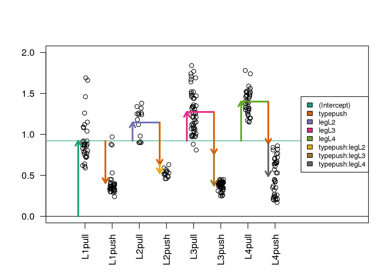
(#fig:spider_interactions2)Diagram of the estimated coefficients in the linear model. In the design with interaction terms, the orange arrow now indicates the push vs. pull difference only for the reference group (L1), while three new arrows (yellow, brown and grey) indicate the additional push vs. pull differences in the non-reference groups (L2, L3 and L4) with respect to the reference group.
5.5.0.2 Contrasts
Again we will show how to combine estimated coefficients from the model using contrasts. For some simple cases, we can use the contrast package. Suppose we want to know the push vs. pull effect for the L2 leg pair samples. We can see from the arrow plot that this is the orange arrow plus the yellow arrow. We can also specify this comparison with the contrast function:
library(contrast) ##Available from CRAN
L2push.vs.pull <- contrast(fitX,
                   list(leg="L2", type = "push"),
                   list(leg="L2", type = "pull"))
L2push.vs.pull
## lm model parameter contrast
##
## Contrast S.E. Lower Upper t df Pr(>|t|)
## -0.618 0.06954 -0.7549 -0.4811 -8.89 274 0coefs[2] + coefs[6] ##we know this is also orange + yellow arrow## typepush
## -0.6185.5.0.3 Differences of differences
The question of whether the push vs. pull difference is different in L2 compared to L1, is answered by a single term in the model: the typepush:legL2 estimated coefficient corresponding to the yellow arrow in the plot. A p-value for whether this coefficient is actually equal to zero can be read off from the table printed with summary(fitX) above. Similarly, we can read off the p-values for the differences of differences for L3 vs. L1 and for L4 vs. L1.
Suppose we want to know if the push vs. pull difference is different in L3 compared to L2. By examining the arrows in the diagram above, we can see that the push vs. pull effect for a leg pair other than L1 is the typepush arrow plus the interaction term for that group.
If we work out the math for comparing across two non-reference leg pairs, this is:
\[ (\mbox{typepush} + \mbox{typepush:legL3}) - (\mbox{typepush} + \mbox{typepush:legL2}) \]
…which simplifies to:
\[ = \mbox{typepush:legL3} - \mbox{typepush:legL2} \]
We can’t make this contrast using the contrast function shown before, but we can make this comparison using the glht (for “general linear hypothesis test”) function from the multcomp package. We need to form a 1-row matrix which has a -1 for the typepush:legL2 coefficient and a +1 for the typepush:legL3 coefficient. We provide this matrix to the linfct (linear function) argument, and obtain a summary table for this contrast of estimated interaction coefficients.
Note that there are other ways to perform contrasts using base R, and this is just our preferred way.
library(multcomp) ##Available from CRAN
C <- matrix(c(0,0,0,0,0,-1,1,0), 1)
L3vsL2interaction <- glht(fitX, linfct=C)
summary(L3vsL2interaction)
##
## Simultaneous Tests for General Linear Hypotheses
##
## Fit: lm(formula = friction ~ type + leg + type:leg, data = spider)
##
## Linear Hypotheses:
## Estimate Std. Error t value Pr(>|t|)
## 1 == 0 -0.2799 0.0789 -3.55 0.00046 ***
## ---
## Signif. codes:
## 0 '***' 0.001 '**' 0.01 '*' 0.05 '.' 0.1 ' ' 1
## (Adjusted p values reported -- single-step method)coefs[7] - coefs[6] ##we know this is also brown - yellow## typepush:legL3
## -0.27995.6 Analysis of Variance
Suppose that we want to know if the push vs. pull difference is different across leg pairs in general. We do not want to compare any two leg pairs in particular, but rather we want to know if the three interaction terms which represent differences in the push vs. pull difference across leg pairs are larger than we would expect them to be if the push vs. pull difference was in fact equal across all leg pairs.
Such a question can be answered by an analysis of variance, which is often abbreviated as ANOVA. ANOVA compares the reduction in the sum of squares of the residuals for models of different complexity. The model with eight coefficients is more complex than the model with five coefficients where we assumed the push vs. pull difference was equal across leg pairs. The least complex model would only use a single coefficient, an intercept. Under certain assumptions we can also perform inference that determines the probability of improvements as large as what we observed. Let’s first print the result of an ANOVA in R and then examine the results in detail:
anova(fitX)## Analysis of Variance Table
##
## Response: friction
## Df Sum Sq Mean Sq F value Pr(>F)
## type 1 42.8 42.8 1179.7 < 2e-16 ***
## leg 3 2.9 1.0 26.9 3.0e-15 ***
## type:leg 3 2.1 0.7 19.3 2.3e-11 ***
## Residuals 274 9.9 0.0
## ---
## Signif. codes:
## 0 '***' 0.001 '**' 0.01 '*' 0.05 '.' 0.1 ' ' 1The first line tells us that adding a variable type (push or pull) to the design is very useful (reduces the sum of squared residuals) compared to a model with only an intercept. We can see that it is useful, because this single coefficient reduces the sum of squares by 42.783. The original sum of squares of the model with just an intercept is:
mu0 <- mean(spider$friction)
(initial.ss <- sum((spider$friction - mu0)^2))
## [1] 57.74Note that this initial sum of squares is just a scaled version of the sample variance:
N <- nrow(spider)
(N - 1) * var(spider$friction)
## [1] 57.74Let’s see exactly how we get this 42.783. We need to calculate the sum of squared residuals for the model with only the type information. We can do this by calculating the residuals, squaring these, summing these within groups and then summing across the groups.
s <- split(spider$friction, spider$type)
after.type.ss <- sum( sapply(s, function(x) {
  residual <- x - mean(x)
  sum(residual^2)
  }) )
The reduction in sum of squared residuals from introducing the type coefficient is therefore:
(type.ss <- initial.ss - after.type.ss)## [1] 42.78Through simple arithmetic, this reduction can be shown to be equivalent to the sum of squared differences between the fitted values for the models with formula ~type and ~1:
sum(sapply(s, length) * (sapply(s, mean) - mu0)^2)## [1] 42.78Keep in mind that the order of terms in the formula, and therefore rows in the ANOVA table, is important: each row considers the reduction in the sum of squared residuals after adding coefficients compared to the model in the previous row.
The other columns in the ANOVA table show the “degrees of freedom” with each row. As the type variable introduced only one term in the model, the Df column has a 1. Because the leg variable introduced three terms in the model (legL2, legL3 and legL4), the Df column has a 3.
Finally, there is a column which lists the F value. The F value is the mean of squares for the inclusion of the terms of interest (the sum of squares divided by the degrees of freedom) divided by the mean squared residuals (from the bottom row):
\[ r_i = Y_i - \hat{Y}_i \]
\[ \mbox{Mean Sq Residuals} = \frac{1}{N - p} \sum_{i=1}^N r_i^2 \]
where \(p\) is the number of coefficients in the model (here eight, including the intercept term).
Under the null hypothesis (the true value of the additional coefficient(s) is 0), we have a theoretical result for what the distribution of the F value will be for each row. The assumptions needed for this approximation to hold are similar to those of the t-distribution approximation we described in earlier chapters. We either need a large sample size so that CLT applies or we need the population data to follow a normal approximation.
As an example of how one interprets these p-values, let’s take the last row type:leg which specifies the three interaction coefficients. Under the null hypothesis that the true value for these three additional terms is actually 0, e.g. \(\beta_{\textrm{push,L2}} = 0, \beta_{\textrm{push,L3}} = 0, \beta_{\textrm{push,L4}} = 0\), then we can calculate the chance of seeing such a large F-value for this row of the ANOVA table. Remember that we are only concerned with large values here, because we have a ratio of sum of squares, the F-value can only be positive. The p-value in the last column for the type:leg row can be interpreted as: under the null hypothesis that there are no differences in the push vs. pull difference across leg pair, this is the probability of an estimated interaction coefficient explaining so much of the observed variance. If this p-value is small, we would consider rejecting the null hypothesis that the push vs. pull difference is the same across leg pairs.
The F distribution has two parameters: one for the degrees of freedom of the numerator (the terms of interest) and one for the denominator (the residuals). In the case of the interaction coefficients row, this is 3, the number of interaction coefficients divided by 274, the number of samples minus the total number of coefficients.
5.6.0.1 A different specification of the same model
Now we show an alternate specification of the same model, wherein we assume that each combination of type and leg has its own mean value (and so that the push vs. pull effect is not the same for each leg pair). This specification is in some ways simpler, as we will see, but it does not allow us to build the ANOVA table as above, because it does not split interaction coefficients out in the same way.
We start by constructing a factor variable with a level for each unique combination of type and leg. We include a 0 + in the formula because we do not want to include an intercept in the model matrix.
##earlier, we defined the 'group' column:
spider$group <- factor(paste0(spider$leg, spider$type))
X <- model.matrix(~ 0 + group, data=spider)
colnames(X)
## [1] "groupL1pull" "groupL1push" "groupL2pull"
## [4] "groupL2push" "groupL3pull" "groupL3push"
## [7] "groupL4pull" "groupL4push"head(X)## groupL1pull groupL1push groupL2pull groupL2push
## 1 1 0 0 0
## 2 1 0 0 0
## 3 1 0 0 0
## 4 1 0 0 0
## 5 1 0 0 0
## 6 1 0 0 0
## groupL3pull groupL3push groupL4pull groupL4push
## 1 0 0 0 0
## 2 0 0 0 0
## 3 0 0 0 0
## 4 0 0 0 0
## 5 0 0 0 0
## 6 0 0 0 0imagemat(X, main="Model matrix for linear model with group variable")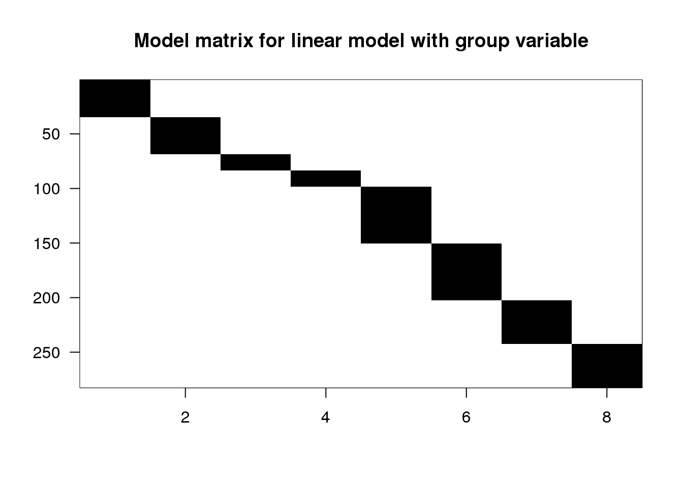
(#fig:matrix_model_image_group_variable)Image of model matrix for linear model with group variable. This model, also with eight terms, gives a unique fitted value for each combination of type and leg.
We can run the linear model with the familiar call:
fitG <- lm(friction ~ 0 + group, data=spider)
summary(fitG)
##
## Call:
## lm(formula = friction ~ 0 + group, data = spider)
##
## Residuals:
## Min 1Q Median 3Q Max
## -0.4638 -0.1074 -0.0111 0.0785 0.7685
##
## Coefficients:
## Estimate Std. Error t value Pr(>|t|)
## groupL1pull 0.9215 0.0327 28.2 <2e-16 ***
## groupL1push 0.4074 0.0327 12.5 <2e-16 ***
## groupL2pull 1.1453 0.0492 23.3 <2e-16 ***
## groupL2push 0.5273 0.0492 10.7 <2e-16 ***
## groupL3pull 1.2738 0.0264 48.2 <2e-16 ***
## groupL3push 0.3760 0.0264 14.2 <2e-16 ***
## groupL4pull 1.4007 0.0301 46.5 <2e-16 ***
## groupL4push 0.4908 0.0301 16.3 <2e-16 ***
## ---
## Signif. codes:
## 0 '***' 0.001 '**' 0.01 '*' 0.05 '.' 0.1 ' ' 1
##
## Residual standard error: 0.19 on 274 degrees of freedom
## Multiple R-squared: 0.96, Adjusted R-squared: 0.959
## F-statistic: 821 on 8 and 274 DF, p-value: <2e-16coefs <- coef(fitG)5.6.0.2 Examining the estimated coefficients
Now we have eight arrows, one for each group. The arrow tips align directly with the mean of each group:
(#fig:estimated_group_variables)Diagram of the estimated coefficients in the linear model, with each term representing the mean of a combination of type and leg.
5.6.0.3 Simple contrasts using the contrast package
While we cannot perform an ANOVA with this formulation, we can easily contrast the estimated coefficients for individual groups using the contrast function:
groupL2push.vs.pull <- contrast(fitG,
                                list(group = "L2push"),
                                list(group = "L2pull"))
groupL2push.vs.pull
## lm model parameter contrast
##
## Contrast S.E. Lower Upper t df Pr(>|t|)
## 1 -0.618 0.06954 -0.7549 -0.4811 -8.89 274 0coefs[4] - coefs[3]## groupL2push
## -0.6185.6.0.4 Differences of differences when there is no intercept
We can also make pair-wise comparisons of the estimated push vs. pull difference across leg pair. For example, if we want to compare the push vs. pull difference in leg pair L3 vs. leg pair L2:
\[ (\mbox{L3push} - \mbox{L3pull}) - (\mbox{L2push} - \mbox{L2pull}) \]
\[ = \mbox{L3 push} + \mbox{L2pull} - \mbox{L3pull} - \mbox{L2push} \]
C <- matrix(c(0,0,1,-1,-1,1,0,0), 1)
groupL3vsL2interaction <- glht(fitG, linfct=C)
summary(groupL3vsL2interaction)
##
## Simultaneous Tests for General Linear Hypotheses
##
## Fit: lm(formula = friction ~ 0 + group, data = spider)
##
## Linear Hypotheses:
## Estimate Std. Error t value Pr(>|t|)
## 1 == 0 -0.2799 0.0789 -3.55 0.00046 ***
## ---
## Signif. codes:
## 0 '***' 0.001 '**' 0.01 '*' 0.05 '.' 0.1 ' ' 1
## (Adjusted p values reported -- single-step method)names(coefs)## [1] "groupL1pull" "groupL1push" "groupL2pull"
## [4] "groupL2push" "groupL3pull" "groupL3push"
## [7] "groupL4pull" "groupL4push"(coefs[6] - coefs[5]) - (coefs[4] - coefs[3])## groupL3push
## -0.27995.7 Collinearity
If an experiment is designed incorrectly we may not be able to estimate the parameters of interest. Similarly, when analyzing data we may incorrectly decide to use a model that can’t be fit. If we are using linear models then we can detect these problems mathematically by looking for collinearity in the design matrix.
5.7.0.1 System of equations example
The following system of equations:
\[ \begin{align*} a+c &=1\\ b-c &=1\\ a+b &=2 \end{align*} \]
has more than one solution since there are an infinite number of triplets that satisfy \(a=1-c, b=1+c\). Two examples are \(a=1,b=1,c=0\) and \(a=0,b=2,c=1\).
5.7.0.2 Matrix algebra approach
The system of equations above can be written like this:
\[ \, \begin{pmatrix} 1&0&1\\ 0&1&-1\\ 1&1&0\\ \end{pmatrix} \begin{pmatrix} a\\ b\\ c \end{pmatrix} = \begin{pmatrix} 1\\ 1\\ 2 \end{pmatrix} \]
Note that the third column is a linear combination of the first two:
\[ \, \begin{pmatrix} 1\\ 0\\ 1 \end{pmatrix} + -1 \begin{pmatrix} 0\\ 1\\ 1 \end{pmatrix} = \begin{pmatrix} 1\\ -1\\ 0 \end{pmatrix} \]
We say that the third column is collinear with the first 2. This implies that the system of equations can be written like this:
\[ \, \begin{pmatrix} 1&0&1\\ 0&1&-1\\ 1&1&0 \end{pmatrix} \begin{pmatrix} a\\ b\\ c \end{pmatrix} = a \begin{pmatrix} 1\\ 0\\ 1 \end{pmatrix} + b \begin{pmatrix} 0\\ 1\\ 1 \end{pmatrix} + c \begin{pmatrix} 1-0\\ 0-1\\ 1-1 \end{pmatrix} \]
\[ =(a+c) \begin{pmatrix} 1\\ 0\\ 1\\ \end{pmatrix} + (b-c) \begin{pmatrix} 0\\ 1\\ 1\\ \end{pmatrix} \]
The third column does not add a constraint and what we really have are three equations and two unknowns: \(a+c\) and \(b-c\). Once we have values for those two quantities, there are an infinity number of triplets that can be used.
5.7.0.3 Collinearity and least squares
Consider a design matrix \(\mathbf{X}\) with two collinear columns. Here we create an extreme example in which one column is the opposite of another:
\[ \mathbf{X} = \begin{pmatrix} \mathbf{1}&\mathbf{X}_1&\mathbf{X}_2&\mathbf{X}_3\\ \end{pmatrix} \mbox{ with, say, } \mathbf{X}_3 = - \mathbf{X}_2 \]
This means that we can rewrite the residuals like this:
\[ \mathbf{Y}- \left\{ \mathbf{1}\beta_0 + \mathbf{X}_1\beta_1 + \mathbf{X}_2\beta_2 + \mathbf{X}_3\beta_3\right\}\\ = \mathbf{Y}- \left\{ \mathbf{1}\beta_0 + \mathbf{X}_1\beta_1 + \mathbf{X}_2\beta_2 - \mathbf{X}_2\beta_3\right\}\\ = \mathbf{Y}- \left\{\mathbf{1}\beta_0 + \mathbf{X}_1 \beta_1 + \mathbf{X}_2(\beta_2 - \beta_3)\right\} \]
and if \(\hat{\beta}_1\), \(\hat{\beta}_2\), \(\hat{\beta}_3\) is a least squares solution, then, for example, \(\hat{\beta}_1\), \(\hat{\beta}_2+1\), \(\hat{\beta}_3+1\) is also a solution.
5.7.0.4 Confounding as an example
Now we will demonstrate how collinearity helps us determine problems with our design using one of the most common errors made in current experimental design: confounding. To illustrate, let’s use an imagined experiment in which we are interested in the effect of four treatments A, B, C and D. We assign two mice to each treatment. After starting the experiment by giving A and B to female mice, we realize there might be a sex effect. We decide to give C and D to males with hopes of estimating this effect. But can we estimate the sex effect? The described design implies the following design matrix:
\[ \, \begin{pmatrix} Sex & A & B & C & D\\ 0 & 1 & 0 & 0 & 0 \\ 0 & 1 & 0 & 0 & 0 \\ 0 & 0 & 1 & 0 & 0 \\ 0 & 0 & 1 & 0 & 0 \\ 1 & 0 & 0 & 1 & 0 \\ 1 & 0 & 0 & 1 & 0 \\ 1 & 0 & 0 & 0 & 1 \\ 1 & 0 & 0 & 0 & 1\\ \end{pmatrix} \]
Here we can see that sex and treatment are confounded. Specifically, the sex column can be written as a linear combination of the C and D matrices.
\[ \, \begin{pmatrix} Sex \\ 0\\ 0 \\ 0 \\ 0 \\ 1\\ 1\\ 1 \\ 1 \\ \end{pmatrix} = \begin{pmatrix} C \\ 0\\ 0\\ 0\\ 0\\ 1\\ 1\\ 0\\ 0\\ \end{pmatrix} + \begin{pmatrix} D \\ 0\\ 0\\ 0\\ 0\\ 0\\ 0\\ 1\\ 1\\ \end{pmatrix} \]
This implies that a unique least squares estimate is not achievable.
5.8 Rank
The rank of a matrix columns is the number of columns that are independent of all the others. If the rank is smaller than the number of columns, then the LSE are not unique. In R, we can obtain the rank of matrix with the function qr, which we will describe in more detail in a following section.
Sex <- c(0,0,0,0,1,1,1,1)
A <-   c(1,1,0,0,0,0,0,0)
B <-   c(0,0,1,1,0,0,0,0)
C <-   c(0,0,0,0,1,1,0,0)
D <-   c(0,0,0,0,0,0,1,1)
X <- model.matrix(~Sex+A+B+C+D-1)
cat("ncol=",ncol(X),"rank=", qr(X)$rank,"\n")
## ncol= 5 rank= 4Here we will not be able to estimate the effect of sex.
5.9 Removing Confounding
This particular experiment could have been designed better. Using the same number of male and female mice, we can easily design an experiment that allows us to compute the sex effect as well as all the treatment effects. Specifically, when we balance sex and treatments, the confounding is removed as demonstrated by the fact that the rank is now the same as the number of columns:
Sex <- c(0,1,0,1,0,1,0,1)
A <-   c(1,1,0,0,0,0,0,0)
B <-   c(0,0,1,1,0,0,0,0)
C <-   c(0,0,0,0,1,1,0,0)
D <-   c(0,0,0,0,0,0,1,1)
X <- model.matrix(~Sex+A+B+C+D-1)
cat("ncol=",ncol(X),"rank=", qr(X)$rank,"\n")
## ncol= 5 rank= 55.10 The QR Factorization (Advanced)
We have seen that in order to calculate the LSE, we need to invert a matrix. In previous sections we used the function solve. However, solve is not a stable solution. When coding LSE computation, we use the QR decomposition.
5.10.0.1 Inverting \(\mathbf{X^\top X}\)
Remember that to minimize the RSS:
\[ (\mathbf{Y}-\mathbf{X}\boldsymbol{\beta})^\top (\mathbf{Y}-\mathbf{X}\boldsymbol{\beta}) \]
We need to solve:
\[ \mathbf{X}^\top \mathbf{X} \boldsymbol{\hat{\beta}} = \mathbf{X}^\top \mathbf{Y} \]
The solution is:
\[ \boldsymbol{\hat{\beta}} = (\mathbf{X}^\top \mathbf{X})^{-1} \mathbf{X}^\top \mathbf{Y} \]
Thus, we need to compute \((\mathbf{X}^\top \mathbf{X})^{-1}\).
5.10.0.2 solve is numerically unstable
To demonstrate what we mean by numerically unstable, we construct an extreme case:
n <- 50;M <- 500
x <- seq(1,M,len=n)
X <- cbind(1,x,x^2,x^3)
colnames(X) <- c("Intercept","x","x2","x3")
beta <- matrix(c(1,1,1,1),4,1)
set.seed(1)
y <- X%*%beta+rnorm(n,sd=1)
The standard R function for inverse gives an error:
solve(crossprod(X)) %*% crossprod(X,y)To see why this happens, look at \((\mathbf{X}^\top \mathbf{X})\)
options(digits=4)
log10(crossprod(X))
## Intercept x x2 x3
## Intercept 1.699 4.098 6.625 9.203
## x 4.098 6.625 9.203 11.810
## x2 6.625 9.203 11.810 14.434
## x3 9.203 11.810 14.434 17.070Note the difference of several orders of magnitude. On a digital computer, we have a limited range of numbers. This makes some numbers seem like 0, when we also have to consider very large numbers. This in turn leads to divisions that are practically divisions by 0 errors.
5.10.0.3 The factorization
The QR factorization is based on a mathematical result that tells us that we can decompose any full rank \(N\times p\) matrix \(\mathbf{X}\) as:
\[ \mathbf{X = QR} \]
with:
- \(\mathbf{Q}\) a \(N \times p\) matrix with \(\mathbf{Q^\top Q=I}\)
- \(\mathbf{R}\) a \(p \times p\) upper triangular matrix.
Upper triangular matrices are very convenient for solving system of equations.
5.10.0.4 Example of upper triangular matrix
In the example below, the matrix on the left is upper triangular: it only has 0s below the diagonal. This facilitates solving the system of equations greatly:
\[ \, \begin{pmatrix} 1&2&-1\\ 0&1&2\\ 0&0&1\\ \end{pmatrix} \begin{pmatrix} a\\ b\\ c\\ \end{pmatrix} = \begin{pmatrix} 6\\ 4\\ 1\\ \end{pmatrix} \]
We immediately know that \(c=1\), which implies that \(b+2=4\). This in turn implies \(b=2\) and thus \(a+4-1=6\) so \(a = 3\). Writing an algorithm to do this is straight-forward for any upper triangular matrix.
5.10.0.5 Finding LSE with QR
If we rewrite the equations of the LSE using \(\mathbf{QR}\) instead of \(\mathbf{X}\) we have:
\[\mathbf{X}^\top \mathbf{X} \boldsymbol{\beta} = \mathbf{X}^\top \mathbf{Y}\]
\[(\mathbf{Q}\mathbf{R})^\top (\mathbf{Q}\mathbf{R}) \boldsymbol{\beta} = (\mathbf{Q}\mathbf{R})^\top \mathbf{Y}\]
\[\mathbf{R}^\top (\mathbf{Q}^\top \mathbf{Q}) \mathbf{R} \boldsymbol{\beta} = \mathbf{R}^\top \mathbf{Q}^\top \mathbf{Y}\]
\[\mathbf{R}^\top \mathbf{R} \boldsymbol{\beta} = \mathbf{R}^\top \mathbf{Q}^\top \mathbf{Y}\]
\[(\mathbf{R}^\top)^{-1} \mathbf{R}^\top \mathbf{R} \boldsymbol{\beta} = (\mathbf{R}^\top)^{-1} \mathbf{R}^\top \mathbf{Q}^\top \mathbf{Y}\]
\[\mathbf{R} \boldsymbol{\beta} = \mathbf{Q}^\top \mathbf{Y}\]
\(\mathbf{R}\) being upper triangular makes solving this more stable. Also, because \(\mathbf{Q}^\top\mathbf{Q}=\mathbf{I}\) , we know that the columns of \(\mathbf{Q}\) are in the same scale which stabilizes the right side.
Now we are ready to find LSE using the QR decomposition. To solve:
\[\mathbf{R} \boldsymbol{\beta} = \mathbf{Q}^\top \mathbf{Y}\]
We use backsolve which takes advantage of the upper triangular nature of \(\mathbf{R}\).
QR <- qr(X)
Q <- qr.Q( QR )
R <- qr.R( QR )
(betahat <- backsolve(R, crossprod(Q,y) ) )
## [,1]
## [1,] 0.9038
## [2,] 1.0066
## [3,] 1.0000
## [4,] 1.0000In practice, we do not need to do any of this due to the built-in solve.qr function:
QR <- qr(X)
(betahat <- solve.qr(QR, y))
## [,1]
## Intercept 0.9038
## x 1.0066
## x2 1.0000
## x3 1.00005.10.0.6 Fitted values
This factorization also simplifies the calculation for fitted values:
\[\mathbf{X}\boldsymbol{\hat{\beta}} = (\mathbf{QR})\mathbf{R}^{-1}\mathbf{Q}^\top \mathbf{y}= \mathbf{Q}\mathbf{Q}^\top\mathbf{y} \]
In R, we simply do the following:
library(rafalib)
mypar(1,1)
plot(x,y)
fitted <- tcrossprod(Q)%*%y
lines(x,fitted,col=2)
5.10.0.7 Standard errors
To obtain the standard errors of the LSE, we note that:
\[(\mathbf{X^\top X})^{-1} = (\mathbf{R^\top Q^\top QR})^{-1} = (\mathbf{R^\top R})^{-1}\]
The function chol2inv is specifically designed to find this inverse. So all we do is the following:
df <- length(y) - QR$rank
sigma2 <- sum((y-fitted)^2)/df
varbeta <- sigma2*chol2inv(qr.R(QR))
SE <- sqrt(diag(varbeta))
cbind(betahat,SE)
## SE
## Intercept 0.9038 4.508e-01
## x 1.0066 7.858e-03
## x2 1.0000 3.662e-05
## x3 1.0000 4.802e-08This gives us identical results to the lm function.
summary(lm(y~0+X))$coef## Estimate Std. Error t value Pr(>|t|)
## XIntercept 0.9038 4.508e-01 2.005e+00 5.089e-02
## Xx 1.0066 7.858e-03 1.281e+02 2.171e-60
## Xx2 1.0000 3.662e-05 2.731e+04 1.745e-167
## Xx3 1.0000 4.802e-08 2.082e+07 4.559e-3005.11 Going Further
Linear models can be extended in many directions. Here are some examples of extensions, which you might come across in analyzing data in the life sciences:
5.11.0.1 Robust linear models
In calculating the solution and its estimated error in the standard linear model, we minimize the squared errors. This involves a sum of squares from all the data points, which means that a few outlier data points can have a large influence on the solution. In addition, the errors are assumed to have constant variance (called homoskedasticity), which might not always hold true (when this is not true, it is called heteroskedasticity). Therefore, methods have been developed to generate more robust solutions, which behave well in the presence of outliers, or when the distributional assumptions are not met. A number of these are mentioned on the robust statistics page on the CRAN website. For more background, there is also a Wikipedia article with references.
5.11.0.2 Generalized linear models
In the standard linear model, we did not make any assumptions about the distribution of \(\mathbf{Y}\), though in some cases we can gain better estimates if we know that \(\mathbf{Y}\) is, for example, restricted to non-negative integers \(0,1,2,\dots\), or restricted to the interval \([0,1]\). A framework for analyzing such cases is referred to as generalized linear models, commonly abbreviated as GLMs. The two key components of the GLM are the link function and a probability distribution. The link function \(g\) connects our familiar matrix product \(\mathbf{X} \boldsymbol{\beta}\) to the \(\mathbf{Y}\) values through:
\[ \textrm{E}(\mathbf{Y}) = g^{-1}( \mathbf{X} \boldsymbol{\beta} ) \]
R includes the function glm which fits GLMs and uses a familiar form as lm. Additional arguments include family, which can be used to specify the distributional assumption for \(\mathbf{Y}\). Some examples of the use of GLMs are shown at the Quick R website. There are a number of references for GLMs on the Wikipedia page.
5.11.0.3 Mixed effects linear models
In the standard linear model, we assumed that the matrix \(\mathbf{X}\) was fixed and not random. For example, we measured the frictional coefficients for each leg pair, and in the push and pull direction. The fact that an observation had a \(1\) for a given column in \(\mathbf{X}\) was not random, but dictated by the experimental design. However, in the father and son heights example, we did not fix the values of the fathers’ heights, but observed these (and likely these were measured with some error). A framework for studying the effect of the randomness for various columns in \(X\) is referred to as mixed effects models, which implies that some effects are fixed and some effects are random. One of the most popular packages in R for fitting linear mixed effects models is lme4 which has an accompanying paper on Fitting Linear Mixed-Effects Models using lme4. There is also a Wikipedia page with more references.
5.11.0.4 Bayesian linear models
The approach presented here assumed \(\boldsymbol{\beta}\) was a fixed (non-random) parameter. We presented methodology that estimates this parameter, along with standard errors that quantify uncertainty, in the estimation process. This is referred to as the frequentist approach. An alternative approach is to assume that \(\boldsymbol{\beta}\) is random and its distribution quantifies our prior beliefs about what \(\boldsymbol{\beta}\) should be. Once we have observed data, then we update our prior beliefs by computing the conditional distribution, referred to as the posterior distribution, of \(\boldsymbol{\beta}\) given the data. This is referred to as the Bayesian approach. For example, once we have computed the posterior distribution of \(\boldsymbol{\beta}\) we can report the most likely outcome of an interval that occurs with high probability (credible interval). In addition, many models can be connected together in what is referred to as a hierarchical model. Note that we provide a brief introduction to Bayesian statistics and hierarchical models in a later chapter. A good reference for Bayesian hierarchical models is Bayesian Data Analysis, and some software for computing Bayesian linear models can be found on the Bayes page on CRAN. Some well known software for computing Bayesian models are stan and BUGS.
5.11.0.5 Penalized linear models
Note that if we include enough parameters in a model we can achieve a residual sum of squares of 0. Penalized linear models introduce a penalty term to the least square equation we minimize. These penalities are typically of the form, \(\lambda \sum_{j=1}^p \|\beta_j\|^k\) and they penalize for large absolute values of \(\beta\) as well as large numbers of parameters. The motivation for this extra term is to avoid over-fitting. To use these models, we need to pick \(\lambda\) which determines how much we penalize. When \(k=2\), this is referred to as ridge regression, Tikhonov regularization, or L2 regularization. When \(k=1\), this is referred to as LASSO or L1 regularization. A good reference for these penalized linear models is the Elements of Statistical Learning textbook, which is available as a free pdf. Some R packages which implement penalized linear models are the lm.ridge function in the MASS package, the lars package, and the glmnet package.