第 4 章矩阵代数

本书中，我们尝试尽可能的使用较少的数学上的符号。因此，我们避免使用微积分来推导统计学概念。然而，在这本书的其余部分，矩阵代数（也被称为线性代数）的数学符号能够极大的促进对数据分析技术的阐述。因此，我们在本章节中来介绍矩阵代数。我们在数据分析过程中这样做，并且使用其主要的应用：线性代数。

我们将使用三组来自于生命科学的数据，一个来自于物理学、一个与遗传学相关、一个来自于小鼠的实验。这三组数据之间差距较大，但是我们仍然使用相同的统计学方法拟合线性模型来结束分析。人们通常使用数据矩阵的语言来对线性模型进行讲解和表述。

4.1 用实例来讲话

4.1.0.1 自由落体

假设你是16世纪的伽利略，正在尝试着描述高空坠物的的速度。你的一个助手爬上比萨的高塔扔下一个球，然后其他的助手记录不同时间时球的位置。让我们利用我们今天所知道的方程式来模拟一些数据，并且增加一些测量误差。

set.seed(1)
g <- 9.8 ##meters per second
n <- 25
tt <- seq(0,3.4,len=n) ##time in secs, note: we use tt because t is a base function
d <- 56.67  - 0.5*g*tt^2 + rnorm(n,sd=1) ##meters

助手们拿着数据找到伽利略告诉他这是他们看到的数据:

mypar()
plot(tt,d,ylab="Distance in meters",xlab="Time in seconds")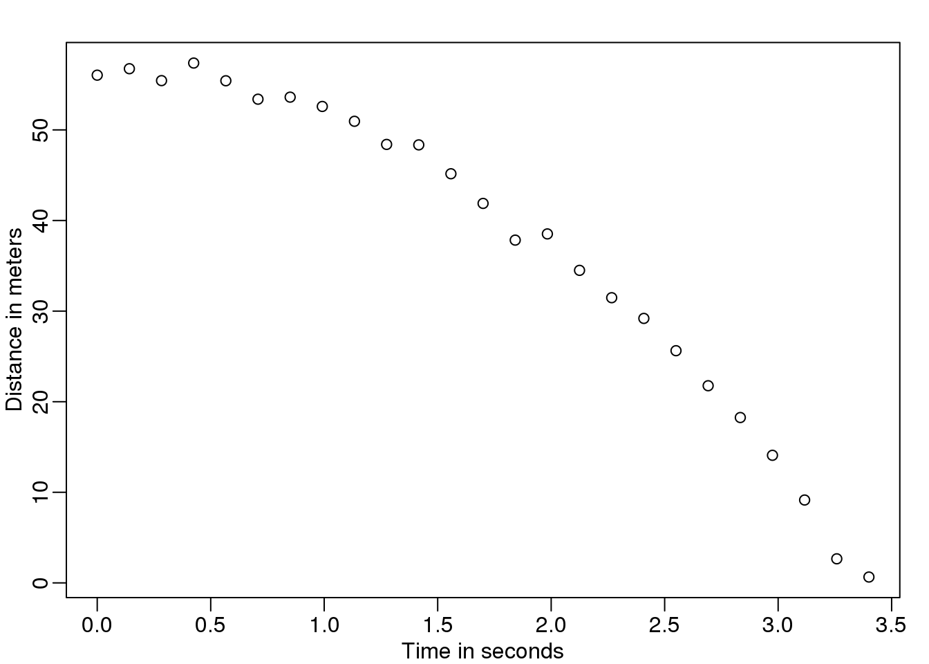

图 4.1: Simulated data for distance travelled versus time of falling object measured with error.

他不知道准确的方程式，但是他通过观察纸上的标绘，推断球的位置应该遵循一个抛物线。因此，他根据这些数据建立了一个模型:

\[ Y_i = \beta_0 + \beta_1 x_i + \beta_2 x_i^2 + \varepsilon_i, i=1,\dots,n \]

其中，\(Y_i\)代表球的位置，\(x_i\)代表观察的时间，\(\varepsilon_i\)表示测量的误差。这是一个线性的模型，因为这是已知数据的线性组合，被成为预测器或者叫做参数位置的协变量(\(\beta\)’s)。

现在假设你是19世纪的弗朗西斯，你收集了一些父亲和儿子之间的身高数据。你猜想，身高是可遗传的，你的数据如下所示:

data(father.son,package="UsingR")
x=father.son$fheight
y=father.son$sheight

看起来像这样：

plot(x,y,xlab="Father's height",ylab="Son's height")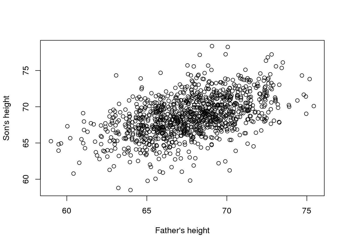

(#fig:galton_data)Galton’s data. Son heights versus father heights.

儿子的身高似乎随着父亲的身高而线性的升高。在这种情况下，可以用一个模型来描述这些数据，如下所示: \[ Y_i = \beta_0 + \beta_1 x_i + \varepsilon_i, i=1,\dots,N \]

这也是一个关于父亲的身高\(x_i\) 和儿子的身高\(Y_i\)的线性模型，对于数据对\(i\)-th和\(\varepsilon_i\)用来解释额外的变量。这里，我们想利用父亲的身高作为一个预测器并且被固定（不是随机的），因此我们使用小写字母。单独的测量误差不能解释在\(\varepsilon_i\)所有的变量。这就表明了这里还存在其他的误差，但是不在所推测的模型中，例如，母亲的身高、遗传的随机性和环境因素。

4.1.0.2 从多个总样中的随机样本

在这里我们从两组不同喂养方式一个是喂养高脂肪数据另一个是喂养正常食物的小鼠中记录老鼠的体重。我们在每一组中随机选择12个小鼠。我们对两组喂养方式是否对小鼠的体重有一定的影响感兴趣。下面是具体的数据。

dat <- read.csv("femaleMiceWeights.csv")
mypar(1,1)
stripchart(Bodyweight~Diet,data=dat,vertical=TRUE,method="jitter",pch=1,main="Mice weights")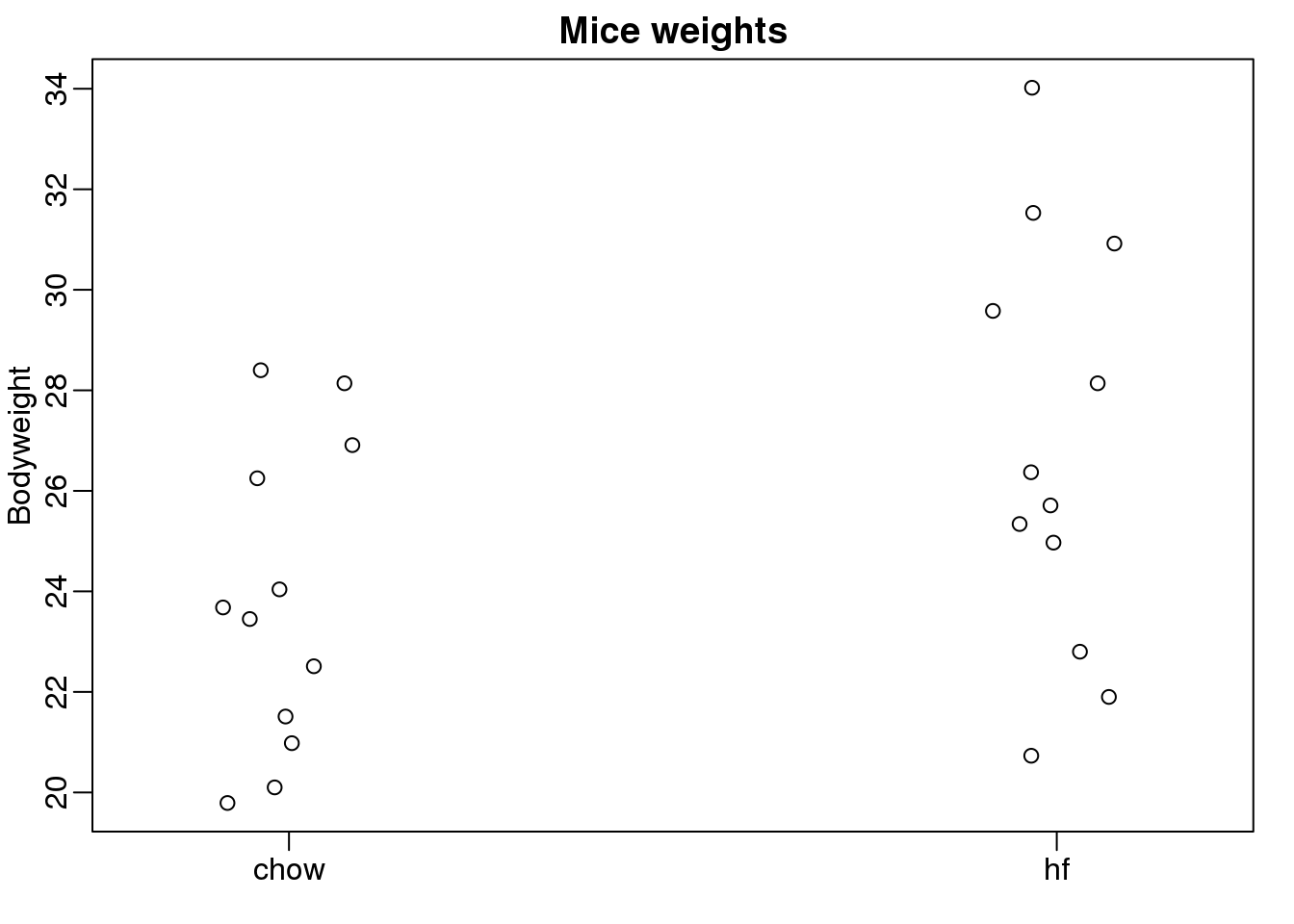

(#fig:mice_weights)Mouse weights under two diets.

我们想要评估在群体之间体重的差异…………………..

\[ Y_i = \beta_0 + \beta_1 x_{i} + \varepsilon_i\]

with \(\beta_0\) the chow diet average weight, \(\beta_1\) the difference between averages, \(x_i = 1\) when mouse \(i\) gets the high fat (hf) diet, \(x_i = 0\) when it gets the chow diet, and \(\varepsilon_i\) explains the differences between mice of the same population.

4.1.0.3 Linear models in general

We have seen three very different examples in which linear models can be used. A general model that encompasses all of the above examples is the following:

\[ Y_i = \beta_0 + \beta_1 x_{i,1} + \beta_2 x_{i,2} + \dots + \beta_2 x_{i,p} + \varepsilon_i, i=1,\dots,n \]

\[ Y_i = \beta_0 + \sum_{j=1}^p \beta_j x_{i,j} + \varepsilon_i, i=1,\dots,n \]

Note that we have a general number of predictors \(p\). Matrix algebra provides a compact language and mathematical framework to compute and make derivations with any linear model that fits into the above framework.

4.1.0.4 Estimating parameters

For the models above to be useful we have to estimate the unknown \(\beta\) s. In the first example, we want to describe a physical process for which we can’t have unknown parameters. In the second example, we better understand inheritance by estimating how much, on average, the father’s height affects the son’s height. In the final example, we want to determine if there is in fact a difference: if \(\beta_1 \neq 0\).

The standard approach in science is to find the values that minimize the distance of the fitted model to the data. The following is called the least squares (LS) equation and we will see it often in this chapter:

\[ \sum_{i=1}^n \left\{ Y_i - \left(\beta_0 + \sum_{j=1}^p \beta_j x_{i,j}\right)\right\}^2 \]

Once we find the minimum, we will call the values the least squares estimates (LSE) and denote them with \(\hat{\beta}\). The quantity obtained when evaluating the least squares equation at the estimates is called the residual sum of squares (RSS). Since all these quantities depend on \(Y\), they are random variables. The \(\hat{\beta}\) s are random variables and we will eventually perform inference on them.

4.1.0.5 Falling object example revisited

Thanks to my high school physics teacher, I know that the equation for the trajectory of a falling object is:

\[d = h_0 + v_0 t - 0.5 \times 9.8 t^2\]

with \(h_0\) and \(v_0\) the starting height and velocity respectively. The data we simulated above followed this equation and added measurement error to simulate n observations for dropping the ball \((v_0=0)\) from the tower of Pisa \((h_0=56.67)\). This is why we used this code to simulate data:

g <- 9.8 ##meters per second
n <- 25
tt <- seq(0,3.4,len=n) ##time in secs, t is a base function
f <- 56.67  - 0.5*g*tt^2
y <-  f + rnorm(n,sd=1)

Here is what the data looks like with the solid line representing the true trajectory:

plot(tt,y,ylab="Distance in meters",xlab="Time in seconds")
lines(tt,f,col=2)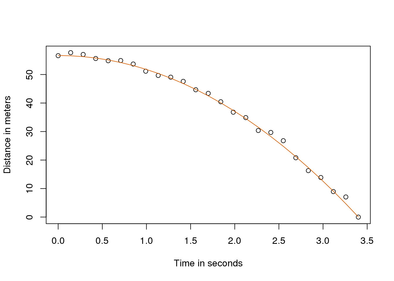

(#fig:simulate_drop_data_with_fit)Fitted model for simulated data for distance travelled versus time of falling object measured with error.

But we were pretending to be Galileo and so we don’t know the parameters in the model. The data does suggest it is a parabola, so we model it as such:

\[ Y_i = \beta_0 + \beta_1 x_i + \beta_2 x_i^2 + \varepsilon_i, i=1,\dots,n \]

How do we find the LSE?

4.1.0.6 The `lm` function

In R we can fit this model by simply using the lm function. We will describe this function in detail later, but here is a preview:

tt2 <-tt^2
fit <- lm(y~tt+tt2)
summary(fit)$coef

##             Estimate Std. Error  t value  Pr(>|t|)
## (Intercept)   57.105     0.4997 114.2817 5.120e-32
## tt            -0.446     0.6807  -0.6553 5.191e-01
## tt2           -4.747     0.1934 -24.5497 1.767e-17

It gives us the LSE, as well as standard errors and p-values.

Part of what we do in this section is to explain the mathematics behind this function.

4.1.0.7 The least squares estimate (LSE)

Let’s write a function that computes the RSS for any vector \(\beta\):

rss <- function(Beta0,Beta1,Beta2){
  r <- y - (Beta0+Beta1*tt+Beta2*tt^2)
  return(sum(r^2))
}

So for any three dimensional vector we get an RSS. Here is a plot of the RSS as a function of \(\beta_2\) when we keep the other two fixed:

Beta2s<- seq(-10,0,len=100)
plot(Beta2s,sapply(Beta2s,rss,Beta0=55,Beta1=0),
     ylab="RSS",xlab="Beta2",type="l")
##Let's add another curve fixing another pair:
Beta2s<- seq(-10,0,len=100)
lines(Beta2s,sapply(Beta2s,rss,Beta0=65,Beta1=0),col=2)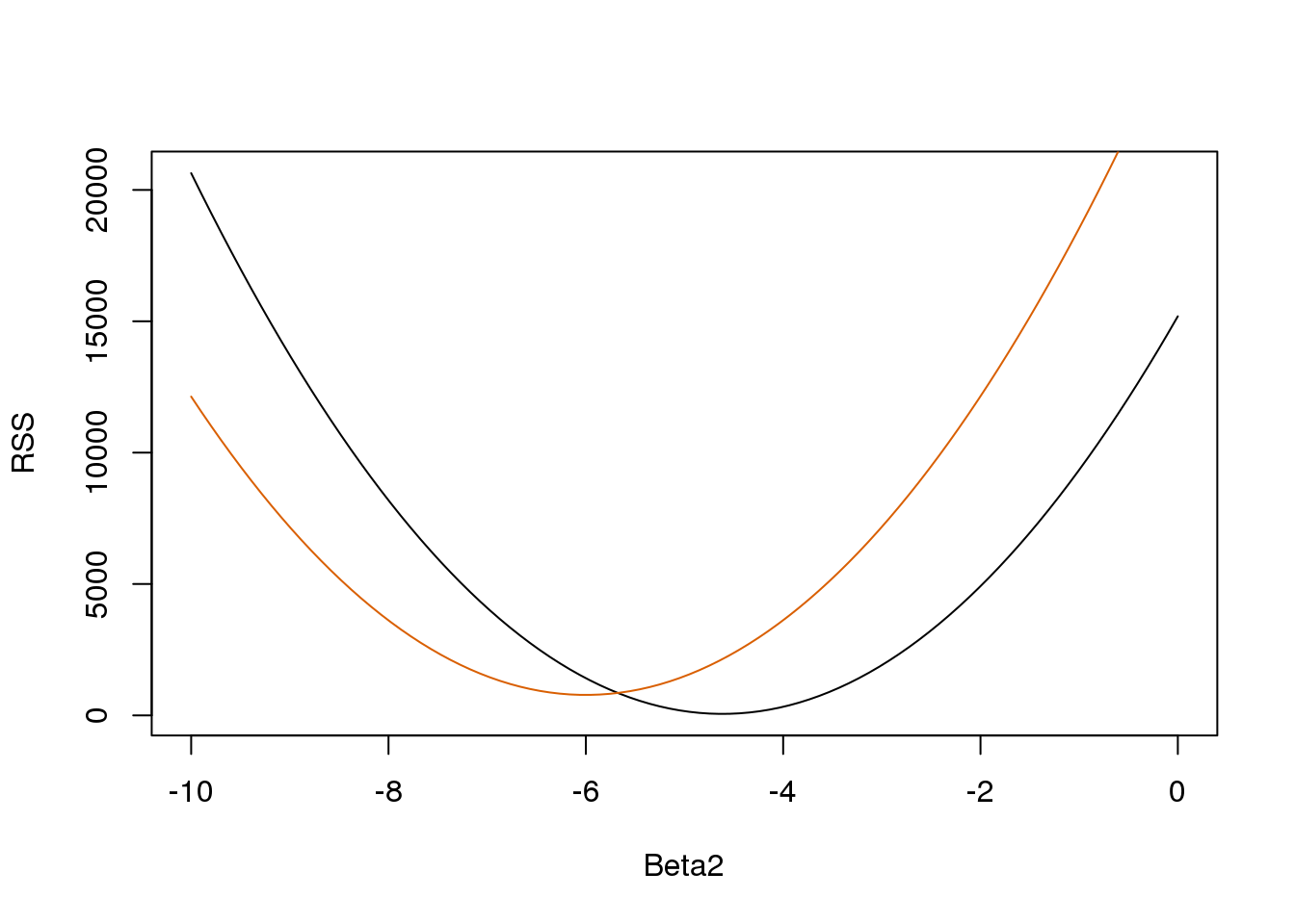

(#fig:rss_versus_estimate)Residual sum of squares obtained for several values of the parameters.

Trial and error here is not going to work. Instead, we can use calculus: take the partial derivatives, set them to 0 and solve. Of course, if we have many parameters, these equations can get rather complex. Linear algebra provides a compact and general way of solving this problem.

4.1.0.8 More on Galton (Advanced)

When studying the father-son data, Galton made a fascinating discovery using exploratory analysis.

Galton’s plot.

He noted that if he tabulated the number of father-son height pairs and followed all the x,y values having the same totals in the table, they formed an ellipse. In the plot above, made by Galton, you see the ellipse formed by the pairs having 3 cases. This then led to modeling this data as correlated bivariate normal which we described earlier:

\[ Pr(X<a,Y<b) = \]

\[ \int_{-\infty}^{a} \int_{-\infty}^{b} \frac{1}{2\pi\sigma_x\sigma_y\sqrt{1-\rho^2}} \exp{ \left\{ \frac{1}{2(1-\rho^2)} \left[\left(\frac{x-\mu_x}{\sigma_x}\right)^2 - 2\rho\left(\frac{x-\mu_x}{\sigma_x}\right)\left(\frac{y-\mu_y}{\sigma_y}\right)+ \left(\frac{y-\mu_y}{\sigma_y}\right)^2 \right] \right\} } \]

We described how we can use math to show that if you keep \(X\) fixed (condition to be \(x\)) the distribution of \(Y\) is normally distributed with mean: \(\mu_x +\sigma_y \rho \left(\frac{x-\mu_x}{\sigma_x}\right)\) and standard deviation \(\sigma_y \sqrt{1-\rho^2}\). Note that \(\rho\) is the correlation between \(Y\) and \(X\), which implies that if we fix \(X=x\), \(Y\) does in fact follow a linear model. The \(\beta_0\) and \(\beta_1\) parameters in our simple linear model can be expressed in terms of \(\mu_x,\mu_y,\sigma_x,\sigma_y\), and \(\rho\).

4.2 Matrix Notation

Here we introduce the basics of matrix notation. Initially this may seem over-complicated, but once we discuss examples, you will appreciate the power of using this notation to both explain and derive solutions, as well as implement them as R code.

4.2.0.1 The language of linear models

Linear algebra notation actually simplifies the mathematical descriptions and manipulations of linear models, as well as coding in R. We will discuss the basics of this notation and then show some examples in R.

The main point of this entire exercise is to show how we can write the models above using matrix notation, and then explain how this is useful for solving the least squares equation. We start by simply defining notation and matrix multiplication, but bear with us since we eventually get back to the practical application.

4.3 Solving Systems of Equations

Linear algebra was created by mathematicians to solve systems of linear equations such as this:

\[ \begin{align*} a + b + c &= 6\\ 3a - 2b + c &= 2\\ 2a + b - c &= 1 \end{align*} \]

It provides very useful machinery to solve these problems generally. We will learn how we can write and solve this system using matrix algebra notation:

\[ \, \begin{pmatrix} 1&1&1\\ 3&-2&1\\ 2&1&-1 \end{pmatrix} \begin{pmatrix} a\\ b\\ c \end{pmatrix} = \begin{pmatrix} 6\\ 2\\ 1 \end{pmatrix} \implies \begin{pmatrix} a\\ b\\ c \end{pmatrix} = \begin{pmatrix} 1&1&1\\ 3&-2&1\\ 2&1&-1 \end{pmatrix}^{-1} \begin{pmatrix} 6\\ 2\\ 1 \end{pmatrix} \]

This section explains the notation used above. It turns out that we can borrow this notation for linear models in statistics as well.

4.4 Vectors, Matrices, and Scalars

In the falling object, father-son heights, and mouse weight examples, the random variables associated with the data were represented by \(Y_1,\dots,Y_n\). We can think of this as a vector. In fact, in R we are already doing this:

data(father.son,package="UsingR")
y=father.son$fheight
head(y)

## [1] 65.05 63.25 64.96 65.75 61.14 63.02

In math we can also use just one symbol. We usually use bold to distinguish it from the individual entries:

\[ \mathbf{Y} = \begin{pmatrix} Y_1\\\ Y_2\\\ \vdots\\\ Y_N \end{pmatrix} \]

For reasons that will soon become clear, default representation of data vectors have dimension \(N\times 1\) as opposed to \(1 \times N\) .

Here we don’t always use bold because normally one can tell what is a matrix from the context.

Similarly, we can use math notation to represent the covariates or predictors. In a case with two predictors we can represent them like this:

\[ \mathbf{X}_1 = \begin{pmatrix} x_{1,1}\\ \vdots\\ x_{N,1} \end{pmatrix} \mbox{ and } \mathbf{X}_2 = \begin{pmatrix} x_{1,2}\\ \vdots\\ x_{N,2} \end{pmatrix} \]

Note that for the falling object example \(x_{1,1}= t_i\) and \(x_{i,1}=t_i^2\) with \(t_i\) the time of the i-th observation. Also, keep in mind that vectors can be thought of as \(N\times 1\) matrices.

For reasons that will soon become apparent, it is convenient to represent these in matrices:

\[ \mathbf{X} = [ \mathbf{X}_1 \mathbf{X}_2 ] = \begin{pmatrix} x_{1,1}&x_{1,2}\\ \vdots\\ x_{N,1}&x_{N,2} \end{pmatrix} \]

This matrix has dimension \(N \times 2\). We can create this matrix in R this way:

n <- 25
tt <- seq(0,3.4,len=n) ##time in secs, t is a base function
X <- cbind(X1=tt,X2=tt^2)
head(X)

##          X1      X2
## [1,] 0.0000 0.00000
## [2,] 0.1417 0.02007
## [3,] 0.2833 0.08028
## [4,] 0.4250 0.18062
## [5,] 0.5667 0.32111
## [6,] 0.7083 0.50174

dim(X)

## [1] 25  2

We can also use this notation to denote an arbitrary number of covariates with the following \(N\times p\) matrix:

\[ \mathbf{X} = \begin{pmatrix} x_{1,1}&\dots & x_{1,p} \\ x_{2,1}&\dots & x_{2,p} \\ & \vdots & \\ x_{N,1}&\dots & x_{N,p} \end{pmatrix} \]

Just as an example, we show you how to make one in R now using matrix instead of cbind:

N <- 100; p <- 5
X <- matrix(1:(N*p),N,p)
head(X)

##      [,1] [,2] [,3] [,4] [,5]
## [1,]    1  101  201  301  401
## [2,]    2  102  202  302  402
## [3,]    3  103  203  303  403
## [4,]    4  104  204  304  404
## [5,]    5  105  205  305  405
## [6,]    6  106  206  306  406

dim(X)

## [1] 100   5

By default, the matrices are filled column by column. The byrow=TRUE argument lets us change that to row by row:

N <- 100; p <- 5
X <- matrix(1:(N*p),N,p,byrow=TRUE)
head(X)

##      [,1] [,2] [,3] [,4] [,5]
## [1,]    1    2    3    4    5
## [2,]    6    7    8    9   10
## [3,]   11   12   13   14   15
## [4,]   16   17   18   19   20
## [5,]   21   22   23   24   25
## [6,]   26   27   28   29   30

Finally, we define a scalar. A scalar is just a number, which we call a scalar because we want to distinguish it from vectors and matrices. We usually use lower case and don’t bold. In the next section, we will understand why we make this distinction.

4.5 Matrix Operations

In a previous section, we motivated the use of matrix algebra with this system of equations:

\[ \begin{align*} a + b + c &= 6\\ 3a - 2b + c &= 2\\ 2a + b - c &= 1 \end{align*} \]

We described how this system can be rewritten and solved using matrix algebra:

\[ \, \begin{pmatrix} 1&1&1\\ 3&-2&1\\ 2&1&-1 \end{pmatrix} \begin{pmatrix} a\\ b\\ c \end{pmatrix} = \begin{pmatrix} 6\\ 2\\ 1 \end{pmatrix} \implies \begin{pmatrix} a\\ b\\ c \end{pmatrix}= \begin{pmatrix} 1&1&1\\ 3&-2&1\\ 2&1&-1 \end{pmatrix}^{-1} \begin{pmatrix} 6\\ 2\\ 1 \end{pmatrix} \]

Having described matrix notation, we will explain the operation we perform with them. For example, above we have matrix multiplication and we also have a symbol representing the inverse of a matrix. The importance of these operations and others will become clear once we present specific examples related to data analysis.

4.5.0.1 Multiplying by a scalar

We start with one of the simplest operations: scalar multiplication. If \(a\) is scalar and \(\mathbf{X}\) is a matrix, then:

\[ \mathbf{X} = \begin{pmatrix} x_{1,1}&\dots & x_{1,p} \\ x_{2,1}&\dots & x_{2,p} \\ & \vdots & \\ x_{N,1}&\dots & x_{N,p} \end{pmatrix} \implies a \mathbf{X} = \begin{pmatrix} a x_{1,1} & \dots & a x_{1,p}\\ a x_{2,1}&\dots & a x_{2,p} \\ & \vdots & \\ a x_{N,1} & \dots & a x_{N,p} \end{pmatrix} \]

R automatically follows this rule when we multiply a number by a matrix using *:

X <- matrix(1:12,4,3)
print(X)

##      [,1] [,2] [,3]
## [1,]    1    5    9
## [2,]    2    6   10
## [3,]    3    7   11
## [4,]    4    8   12

a <- 2
print(a*X)

##      [,1] [,2] [,3]
## [1,]    2   10   18
## [2,]    4   12   20
## [3,]    6   14   22
## [4,]    8   16   24

4.5.0.2 The transpose

The transpose is an operation that simply changes columns to rows. We use a \(\top\) to denote a transpose. The technical definition is as follows: if X is as we defined it above, here is the transpose which will be \(p\times N\):

\[ \mathbf{X} = \begin{pmatrix} x_{1,1}&\dots & x_{1,p} \\ x_{2,1}&\dots & x_{2,p} \\ & \vdots & \\ x_{N,1}&\dots & x_{N,p} \end{pmatrix} \implies \mathbf{X}^\top = \begin{pmatrix} x_{1,1}&\dots & x_{p,1} \\ x_{1,2}&\dots & x_{p,2} \\ & \vdots & \\ x_{1,N}&\dots & x_{p,N} \end{pmatrix} \]

In R we simply use t:

X <- matrix(1:12,4,3)
X

##      [,1] [,2] [,3]
## [1,]    1    5    9
## [2,]    2    6   10
## [3,]    3    7   11
## [4,]    4    8   12

t(X)

##      [,1] [,2] [,3] [,4]
## [1,]    1    2    3    4
## [2,]    5    6    7    8
## [3,]    9   10   11   12

4.5.0.3 Matrix multiplication

We start by describing the matrix multiplication shown in the original system of equations example:

\[ \begin{align*} a + b + c &=6\\ 3a - 2b + c &= 2\\ 2a + b - c &= 1 \end{align*} \]

What we are doing is multiplying the rows of the first matrix by the columns of the second. Since the second matrix only has one column, we perform this multiplication by doing the following:

\[ \, \begin{pmatrix} 1&1&1\\ 3&-2&1\\ 2&1&-1 \end{pmatrix} \begin{pmatrix} a\\ b\\ c \end{pmatrix}= \begin{pmatrix} a + b + c \\ 3a - 2b + c \\ 2a + b - c \end{pmatrix} \]

Here is a simple example. We can check to see if abc=c(3,2,1) is a solution:

X  <- matrix(c(1,3,2,1,-2,1,1,1,-1),3,3)
abc <- c(3,2,1) #use as an example
rbind( sum(X[1,]*abc), sum(X[2,]*abc), sum(X[3,]*abc))

##      [,1]
## [1,]    6
## [2,]    6
## [3,]    7

We can use the %*% to perform the matrix multiplication and make this much more compact:

X%*%abc

##      [,1]
## [1,]    6
## [2,]    6
## [3,]    7

We can see that c(3,2,1) is not a solution as the answer here is not the required c(6,2,1).

To get the solution, we will need to invert the matrix on the left, a concept we learn about below.

Here is the general definition of matrix multiplication of matrices \(A\) and \(X\):

\[ \mathbf{AX} = \begin{pmatrix} a_{1,1} & a_{1,2} & \dots & a_{1,N}\\ a_{2,1} & a_{2,2} & \dots & a_{2,N}\\ & & \vdots & \\ a_{M,1} & a_{M,2} & \dots & a_{M,N} \end{pmatrix} \begin{pmatrix} x_{1,1}&\dots & x_{1,p} \\ x_{2,1}&\dots & x_{2,p} \\ & \vdots & \\ x_{N,1}&\dots & x_{N,p} \end{pmatrix} \]

\[ = \begin{pmatrix} \sum_{i=1}^N a_{1,i} x_{i,1} & \dots & \sum_{i=1}^N a_{1,i} x_{i,p}\\ & \vdots & \\ \sum_{i=1}^N a_{M,i} x_{i,1} & \dots & \sum_{i=1}^N a_{M,i} x_{i,p} \end{pmatrix} \]

You can only take the product if the number of columns of the first matrix \(A\) equals the number of rows of the second one \(X\). Also, the final matrix has the same row numbers as the first \(A\) and the same column numbers as the second \(X\). After you study the example below, you may want to come back and re-read the sections above.

4.5.0.4 The identity matrix

The identity matrix is analogous to the number 1: if you multiply the identity matrix by another matrix, you get the same matrix. For this to happen, we need it to be like this:

\[ \mathbf{I} = \begin{pmatrix} 1&0&0&\dots&0&0\\ 0&1&0&\dots&0&0\\ 0&0&1&\dots&0&0\\ \vdots &\vdots & \vdots&\ddots&\vdots&\vdots\\ 0&0&0&\dots&1&0\\ 0&0&0&\dots&0&1 \end{pmatrix} \]

By this definition, the identity always has to have the same number of rows as columns or be what we call a square matrix.

If you follow the matrix multiplication rule above, you notice this works out:

\[ \mathbf{XI} = \begin{pmatrix} x_{1,1} & \dots & x_{1,p}\\ & \vdots & \\ x_{N,1} & \dots & x_{N,p} \end{pmatrix} \begin{pmatrix} 1&0&0&\dots&0&0\\ 0&1&0&\dots&0&0\\ 0&0&1&\dots&0&0\\ & & &\vdots& &\\ 0&0&0&\dots&1&0\\ 0&0&0&\dots&0&1 \end{pmatrix} = \begin{pmatrix} x_{1,1} & \dots & x_{1,p}\\ & \vdots & \\ x_{N,1} & \dots & x_{N,p} \end{pmatrix} \]

In R you can form an identity matrix this way:

n <- 5 #pick dimensions
diag(n)

##      [,1] [,2] [,3] [,4] [,5]
## [1,]    1    0    0    0    0
## [2,]    0    1    0    0    0
## [3,]    0    0    1    0    0
## [4,]    0    0    0    1    0
## [5,]    0    0    0    0    1

4.5.0.5 The inverse

The inverse of matrix \(X\), denoted with \(X^{-1}\), has the property that, when multiplied, gives you the identity \(X^{-1}X=I\). Of course, not all matrices have inverses. For example, a \(2\times 2\) matrix with 1s in all its entries does not have an inverse.

As we will see when we get to the section on applications to linear models, being able to compute the inverse of a matrix is quite useful. A very convenient aspect of R is that it includes a predefined function solve to do this. Here is how we would use it to solve the linear of equations:

X <- matrix(c(1,3,2,1,-2,1,1,1,-1),3,3)
y <- matrix(c(6,2,1),3,1)
solve(X)%*%y #equivalent to solve(X,y)

##      [,1]
## [1,]    1
## [2,]    2
## [3,]    3

Please note that solve is a function that should be used with caution as it is not generally numerically stable. We explain this in much more detail in the QR factorization section.

4.6 Examples

Now we are ready to see how matrix algebra can be useful when analyzing data. We start with some simple examples and eventually arrive at the main one: how to write linear models with matrix algebra notation and solve the least squares problem.

4.6.0.1 The average

To compute the sample average and variance of our data, we use these formulas \(\bar{Y}=\frac{1}{N} Y_i\) and \(\mbox{var}(Y)=\frac{1}{N} \sum_{i=1}^N (Y_i - \bar{Y})^2\). We can represent these with matrix multiplication. First, define this \(N \times 1\) matrix made just of 1s:

\[ A=\begin{pmatrix} 1\\ 1\\ \vdots\\ 1 \end{pmatrix} \]

This implies that:

\[ \frac{1}{N} \mathbf{A}^\top Y = \frac{1}{N} \begin{pmatrix}1&1&\dots&1\end{pmatrix} \begin{pmatrix} Y_1\\ Y_2\\ \vdots\\ Y_N \end{pmatrix}= \frac{1}{N} \sum_{i=1}^N Y_i = \bar{Y} \]

Note that we are multiplying by the scalar \(1/N\). In R, we multiply matrix using %*%:

data(father.son,package="UsingR")
y <- father.son$sheight
print(mean(y))

## [1] 68.68

N <- length(y)
Y<- matrix(y,N,1)
A <- matrix(1,N,1)
barY=t(A)%*%Y / N

print(barY)

##       [,1]
## [1,] 68.68

4.6.0.2 The variance

As we will see later, multiplying the transpose of a matrix with another is very common in statistics. In fact, it is so common that there is a function in R:

barY=crossprod(A,Y) / N
print(barY)

##       [,1]
## [1,] 68.68

For the variance, we note that if:

\[ \mathbf{r}\equiv \begin{pmatrix} Y_1 - \bar{Y}\\ \vdots\\ Y_N - \bar{Y} \end{pmatrix}, \,\, \frac{1}{N} \mathbf{r}^\top\mathbf{r} = \frac{1}{N}\sum_{i=1}^N (Y_i - \bar{Y})^2 \]

In R, if you only send one matrix into crossprod, it computes: \(r^\top r\) so we can simply type:

r <- y - barY

## Warning in y - barY: Recycling array of length 1 in vector-array arithmetic is deprecated.
##   Use c() or as.vector() instead.

crossprod(r)/N

##       [,1]
## [1,] 7.915

Which is almost equivalent to:

library(rafalib)
popvar(y)

## [1] 7.915

4.6.0.3 Linear models

Now we are ready to put all this to use. Let’s start with Galton’s example. If we define these matrices:

\[ \mathbf{Y} = \begin{pmatrix} Y_1\\ Y_2\\ \vdots\\ Y_N \end{pmatrix} , \mathbf{X} = \begin{pmatrix} 1&x_1\\ 1&x_2\\ \vdots\\ 1&x_N \end{pmatrix} , \mathbf{\beta} = \begin{pmatrix} \beta_0\\ \beta_1 \end{pmatrix} \mbox{ and } \mathbf{\varepsilon} = \begin{pmatrix} \varepsilon_1\\ \varepsilon_2\\ \vdots\\ \varepsilon_N \end{pmatrix} \]

Then we can write the model:

\[ Y_i = \beta_0 + \beta_1 x_i + \varepsilon_i, i=1,\dots,N \]

as:

\[ \, \begin{pmatrix} Y_1\\ Y_2\\ \vdots\\ Y_N \end{pmatrix} = \begin{pmatrix} 1&x_1\\ 1&x_2\\ \vdots\\ 1&x_N \end{pmatrix} \begin{pmatrix} \beta_0\\ \beta_1 \end{pmatrix} + \begin{pmatrix} \varepsilon_1\\ \varepsilon_2\\ \vdots\\ \varepsilon_N \end{pmatrix} \]

or simply:

\[ \mathbf{Y}=\mathbf{X}\boldsymbol{\beta}+\boldsymbol{\varepsilon} \]

which is a much simpler way to write it.

The least squares equation becomes simpler as well since it is the following cross-product:

\[ (\mathbf{Y}-\mathbf{X}\boldsymbol{\beta})^\top (\mathbf{Y}-\mathbf{X}\boldsymbol{\beta}) \]

So now we are ready to determine which values of \(\beta\) minimize the above, which we can do using calculus to find the minimum.

4.6.0.4 Advanced: Finding the minimum using calculus

There are a series of rules that permit us to compute partial derivative equations in matrix notation. By equating the derivative to 0 and solving for the \(\beta\), we will have our solution. The only one we need here tells us that the derivative of the above equation is:

\[ 2 \mathbf{X}^\top (\mathbf{Y} - \mathbf{X} \boldsymbol{\hat{\beta}})=0 \]

\[ \mathbf{X}^\top \mathbf{X} \boldsymbol{\hat{\beta}} = \mathbf{X}^\top \mathbf{Y} \]

\[ \boldsymbol{\hat{\beta}} = (\mathbf{X}^\top \mathbf{X})^{-1} \mathbf{X}^\top \mathbf{Y} \]

and we have our solution. We usually put a hat on the \(\beta\) that solves this, \(\hat{\beta}\) , as it is an estimate of the “real” \(\beta\) that generated the data.

Remember that the least squares are like a square (multiply something by itself) and that this formula is similar to the derivative of \(f(x)^2\) being \(2f(x)f\prime (x)\).

4.6.0.5 Finding LSE in R

Let’s see how it works in R:

data(father.son,package="UsingR")
x=father.son$fheight
y=father.son$sheight
X <- cbind(1,x)
betahat <- solve( t(X) %*% X ) %*% t(X) %*% y
###or
betahat <- solve( crossprod(X) ) %*% crossprod( X, y )

Now we can see the results of this by computing the estimated \(\hat{\beta}_0+\hat{\beta}_1 x\) for any value of \(x\):

newx <- seq(min(x),max(x),len=100)
X <- cbind(1,newx)
fitted <- X%*%betahat
plot(x,y,xlab="Father's height",ylab="Son's height")
lines(newx,fitted,col=2)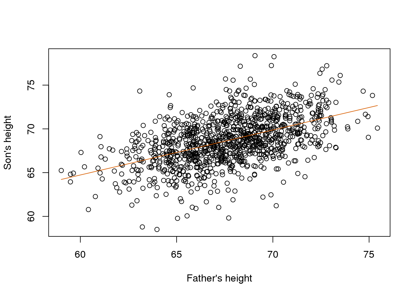

(#fig:galton_regression_line)Galton’s data with fitted regression line.

This \(\hat{\boldsymbol{\beta}}=(\mathbf{X}^\top \mathbf{X})^{-1} \mathbf{X}^\top \mathbf{Y}\) is one of the most widely used results in data analysis. One of the advantages of this approach is that we can use it in many different situations. For example, in our falling object problem:

set.seed(1)
g <- 9.8 #meters per second
n <- 25
tt <- seq(0,3.4,len=n) #time in secs, t is a base function
d <- 56.67  - 0.5*g*tt^2 + rnorm(n,sd=1)

Notice that we are using almost the same exact code:

X <- cbind(1,tt,tt^2)
y <- d
betahat <- solve(crossprod(X))%*%crossprod(X,y)
newtt <- seq(min(tt),max(tt),len=100)
X <- cbind(1,newtt,newtt^2)
fitted <- X%*%betahat
plot(tt,y,xlab="Time",ylab="Height")
lines(newtt,fitted,col=2)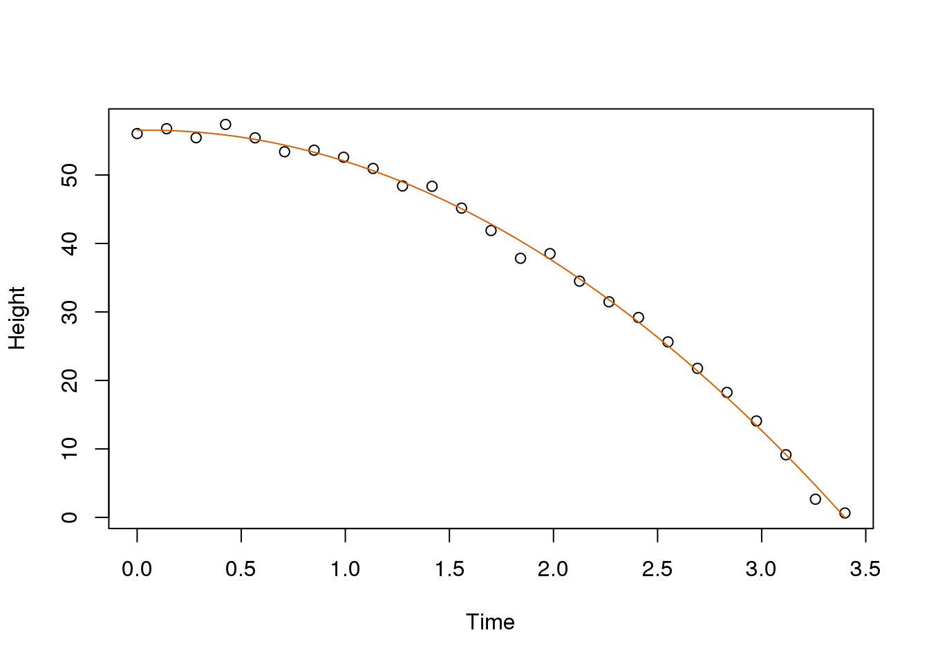

(#fig:gravity_with_fitted_parabola)Fitted parabola to simulated data for distance travelled versus time of falling object measured with error.

And the resulting estimates are what we expect:

betahat

##       [,1]
##    56.5317
## tt  0.5014
##    -5.0386

The Tower of Pisa is about 56 meters high. Since we are just dropping the object there is no initial velocity, and half the constant of gravity is 9.8/2=4.9 meters per second squared.

4.6.0.6 The `lm` Function

R has a very convenient function that fits these models. We will learn more about this function later, but here is a preview:

X <- cbind(tt,tt^2)
fit=lm(y~X)
summary(fit)

## 
## Call:
## lm(formula = y ~ X)
## 
## Residuals:
##    Min     1Q Median     3Q    Max 
## -2.530 -0.488  0.254  0.656  1.546 
## 
## Coefficients:
##             Estimate Std. Error t value Pr(>|t|)    
## (Intercept)   56.532      0.545  103.70   <2e-16 ***
## Xtt            0.501      0.743    0.68     0.51    
## X             -5.039      0.211  -23.88   <2e-16 ***
## ---
## Signif. codes:  
## 0 '***' 0.001 '**' 0.01 '*' 0.05 '.' 0.1 ' ' 1
## 
## Residual standard error: 0.982 on 22 degrees of freedom
## Multiple R-squared:  0.997,  Adjusted R-squared:  0.997 
## F-statistic: 4.02e+03 on 2 and 22 DF,  p-value: <2e-16

Note that we obtain the same values as above.

4.6.0.7 Summary

We have shown how to write linear models using linear algebra. We are going to do this for several examples, many of which are related to designed experiments. We also demonstrated how to obtain least squares estimates. Nevertheless, it is important to remember that because \(y\) is a random variable, these estimates are random as well. In a later section, we will learn how to compute standard error for these estimates and use this to perform inference.

第 4 章 矩阵代数