第 7 章 统计模型

All models are wrong, but some are useful. -George E. P. Box

  当我们在文献里面看见P值时, 这意味着作者采用了某种概率分布来对零假设建模。 很多时候,使用哪种概率分布是相对比较简单的。例如,在茶品鉴中我们可以使用简单的概率计算来确定零假设。大多数的P值或者是样本均值或者是从线性模型的最小平方。??????

  中心极限定理(CLT)的理论基础保证了近似(approximation)的准确性。但是我们并不能总是使用这种近似,比如当样本太小的时候。前面我们讲到了当总体符合正太分布时,样本均值可以近似成t分布。但是,这种假设并没有理论基础。现在我们开始建模。我们从经验中知道身高是一个很好的例子用来建模。

  但是这并不代表我们调查的每一个数据集都服从正态分布。比如一些不符合正态分布的例子有:掷硬币,中奖人数以及美国人的收入.正态分布并不是唯一的可以用来建模的参数分布。这里我们会简单的解少一些常见的参数分布以及它们在生命科学领域的应用。我们主要集中在模型。因此,我们也需要介绍贝叶斯统计的基本知识。如果你想获得对概率模型和参数分布更深入的描述,请参考教科书数据(Mathematical Statistics and Data Analysis)。

7.1 二项分布 (The Binomial Distribution)

  第一个我们要介绍的分布是二项分布。二项分布给出的是在\(N\)次试验中观测到\(S=k\)成功的概率。

\[ \mbox{Pr}(S=k) = {N \choose k}p^k (1-p)^{N-k} \]

  其中\(p\)是成功事件的概率。最经典的例子是掷\(N\)次硬币。掷硬币的例子中,\(N\)是掷硬币的次数,而\(p=0.5\),表示观测到正面的概率。

  [XXneedattention]需要指出的是\(S/N\)是独立随机变量的均值,因此中心极限定律告诉我们在\(N\)很大时\(S\)近似正太分布。最近,二项分布被用于下代测序技术中的变异鉴定和基因型分型中。该分布的一个特殊性是泊松分布可近似为二项分布,接下来我们来介绍泊松分布。

7.2 泊松分布 (The Poisson Distribution)

  彩票中奖人数服从二项分布(我们假设每个人只买一张彩票)。试验的次数\(N\)是买彩票的人数,通常这个数会比较大。但是,彩票中奖人数却是在0至3之间,因此正态分布近似并不成立。为什么中心极限定律并不成立呢?

p=10^-7 ##1 in 10,000,0000 chances of winning
N=5*10^6 ##5,000,000 tickets bought
winners=rbinom(1000,N,p) ##1000 is the number of different lotto draws
tab=table(winners)
plot(tab)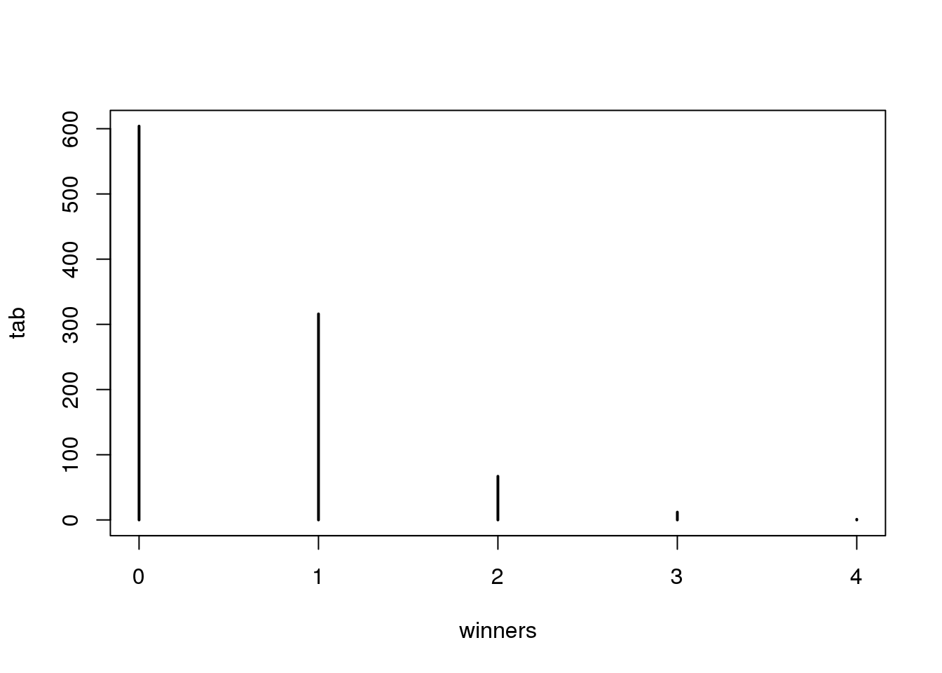

(#fig:lottery_winners_outcomes)Number of people that win the lottery obtained from Monte Carlo simulation.

prop.table(tab)

## winners
##     0     1     2     3     4 
## 0.604 0.316 0.067 0.012 0.001

  在这种情况下,\(N\)非常大,而\(p\)又足够小从而使\(N \times p\)(这里称它为\(\lambda\))成为一个从0到某个值(例如10)的数。 这个时候\(S\)可被看成是服从泊松分布.泊松分布可以用一个简单的公式来表示:

\[ \mbox{Pr}(S=k)=\frac{\lambda^k e^{-\lambda}}{k!} \]

  泊松分布在RNA-seq数据的分析中被广泛的使用。因为在RNA-seq数据中我们有成千上万个基因,而大多数的基因的表达量只占总表达量的一小部分。泊松分布比较适合这种情况。

  为什么泊松分布能帮助我们呢？ 其中一个作用是泊松分布为我们提供了在实践中经常会用到的统计属性。例如，在在一对处理和对照组的RNA-seq数据中，我们想鉴定倍数变化最明显的基因。泊松分布模型中的一种情况是，在零假设为没有差异的时候，倍数变化的变异程度取决于基因的表达丰度。

N=10000##number of genes
lambdas=2^seq(1,16,len=N) ##these are the true abundances of genes
y=rpois(N,lambdas)##note that the null hypothesis is true for all genes
x=rpois(N,lambdas) 
ind=which(y>0 & x>0)##make sure no 0s due to ratio and log

library(rafalib)
splot(log2(lambdas),log2(y/x),subset=ind)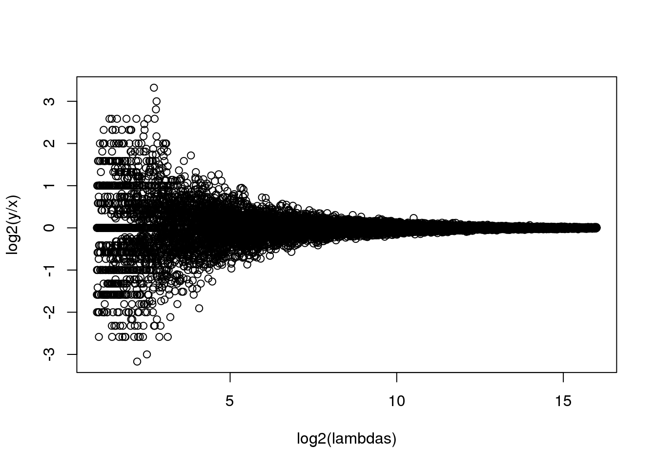

(#fig:rna_seq_simulation)MA plot of simulated RNA-seq data. Replicated measurements follow a Poisson distribution.

  比较小的lambda有更大的变异。如果我们认为倍数变化大于或者等于2的基因是差异表达基因的话,那么对于低丰度的基因,假阳性的数目将会相当的高。

  在这一节，我们将使用下面的数据：

library(parathyroidSE) ##available from Bioconductor
data(parathyroidGenesSE)
se <- parathyroidGenesSE

  这个数据保存在一个SummarizedExperiment对象中，这里我们不对其进项详述。你只需要知道SummarizedExperiment对象中包含一个矩阵数据，这个矩阵中每一列是一个基因，每一行是一个样本。我们可以使用函数assay来提取这个矩阵。在这个矩阵中，每一个单元格是对应的样本中比对到对应基因的短序列的个数（read count）。利用这个数据我们得到了一个和模拟数据相似的一个图，这表明泊松模型预测的结果和我们真实实验数据得到的结果一致。

  在R代码中，ind=which(y>0 & x>0)的作用是将x和y中均大于零的索引值（index）提出来。在使用splot时只对这些数据进行作图，因为这些0的行会在进行除法和对数运算时会导致报错。因为这里我们没有\(\lambda\)，我们使用(log2(x)+log2(y))/2作为对\(\lambda\)的估算。

x <- assay(se)[,23]
y <- assay(se)[,24]
ind=which(y>0 & x>0)##make sure no 0s due to ratio and log 
splot((log2(x)+log2(y))/2,log(x/y),subset=ind)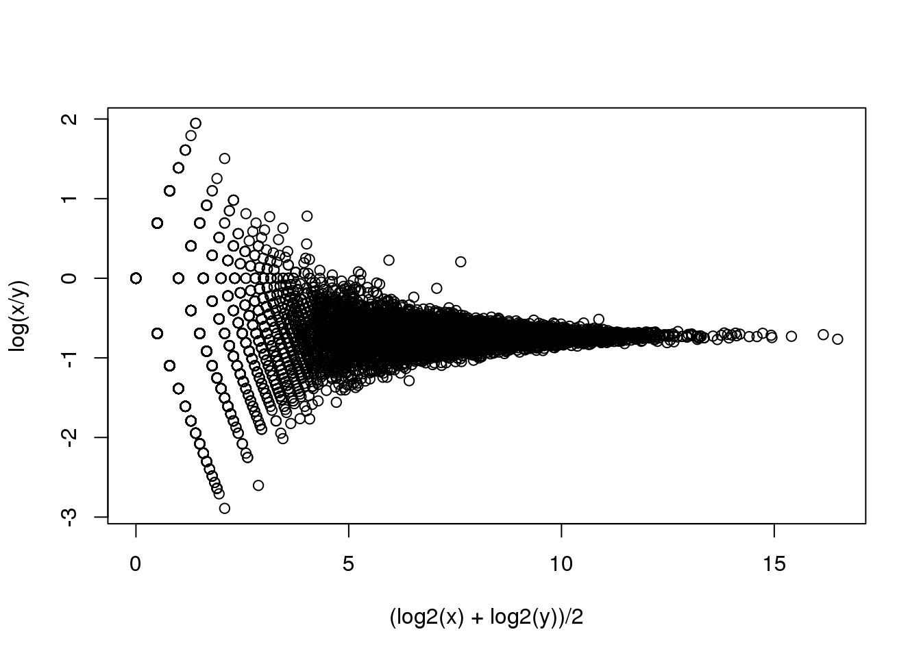

(#fig:RNA-seq_MAplot)MA plot of replicated RNA-seq data.

  如果我们选取其中四个样本中计算其方差。从图中我们可以看到这些方差与泊松分布中预测的值相比高很多（在泊松分布模型中变量的均值和方差相等，均为\(\lambda\)）。假设大多数的基因在不同的样本中是差异表达的，那么如果泊松分布模型是合适的话，我们应该在图中看到横坐标均值和纵坐标方差与图中的实线拟合。

library(rafalib)
library(matrixStats)

vars=rowVars(assay(se)[,c(2,8,16,21)]) ##we know these are four
means=rowMeans(assay(se)[,c(2,8,16,21)]) ##different individuals

splot(means,vars,log="xy",subset=which(means>0&vars>0)) ##plot a subset of data
abline(0,1,col=2,lwd=2)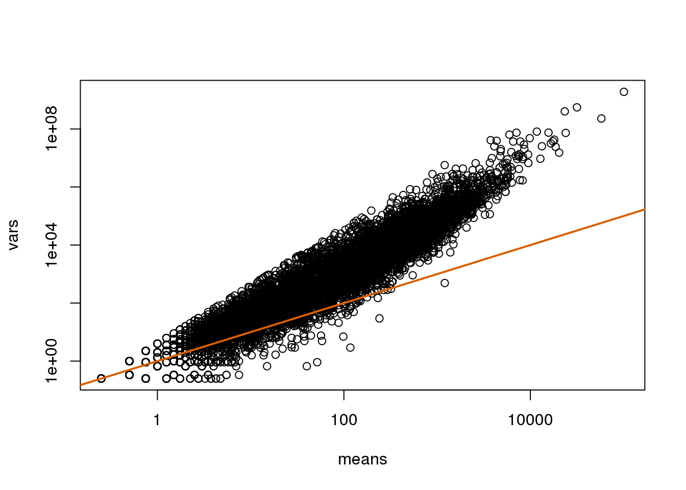

(#fig:var_vs_mean)Variance versus mean plot. Summaries were obtained from the RNA-seq data.

  横坐标均值和纵坐标方差与图中的实线并不拟合是因为图中的变异中包含了生物学变异，而泊松分布模型并不能包含这些生物学变异。负二项分布可以结合泊松分布变异和生物学变异，因此更适合这种生物学数据。负二项分布有两个参数从而可以更灵活的处理短序列计数的数据。如果你想了解跟多的关于使用负二项分布来对RNA-seq数据建模的内容，可以参考这篇文献。泊松分布是负二项分布的一个特例。

7.3 最大似然估计

  为了能解释最大似然估计的概念，这里我们使用一个相对比较简单的数据。该数据中包含了HMCV（人巨细胞病毒：human cytomegalovirus）基因组中的回文序列。我们读取这些回文序列的位置，然后计算每4k区段内的回文序列数目。

datadir="http://www.biostat.jhsph.edu/bstcourse/bio751/data"
x=read.csv(file.path(datadir,"hcmv.csv"))[,2]

breaks=seq(0,4000*round(max(x)/4000),4000)
tmp=cut(x,breaks)
counts=table(tmp)

library(rafalib)
mypar(1,1)
hist(counts)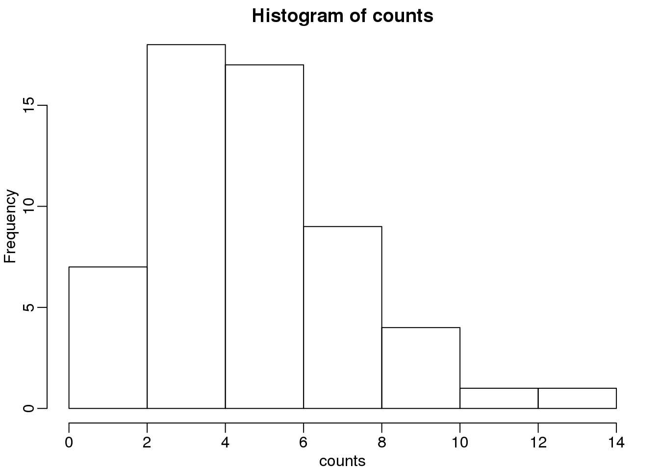

(#fig:palindrome_count_histogram)Palindrome count histogram.

  这些回文序列的个数看起来确实服从泊松分布。但是，在这个数据中的\(\lambda\)是多少呢？最常用的一种方法是最大似然估计。为了找到最大似然估计，我们假设这些数据是独立的，我们观测到这些个数的概率是：

\[ \Pr(X_1=k_1,\dots,X_n=k_n;\lambda) = \prod_{i=1}^n \lambda^{k_i} / k_i! \exp ( -\lambda) \]

  最大似然估计就是找到能够使上面的公式最大的\(\lambda\)值。

\[ \mbox{L}(\lambda; X_1=k_1,\dots,X_n=k_1)=\exp\left\{\sum_{i=1}^n \log \Pr(X_i=k_i;\lambda)\right\} \]

  在实践中，计算

l<-function(lambda) sum(dpois(counts,lambda,log=TRUE)) 

lambdas<-seq(3,7,len=100)
ls <- exp(sapply(lambdas,l))

plot(lambdas,ls,type="l")

mle=optimize(l,c(0,10),maximum=TRUE)
abline(v=mle$maximum)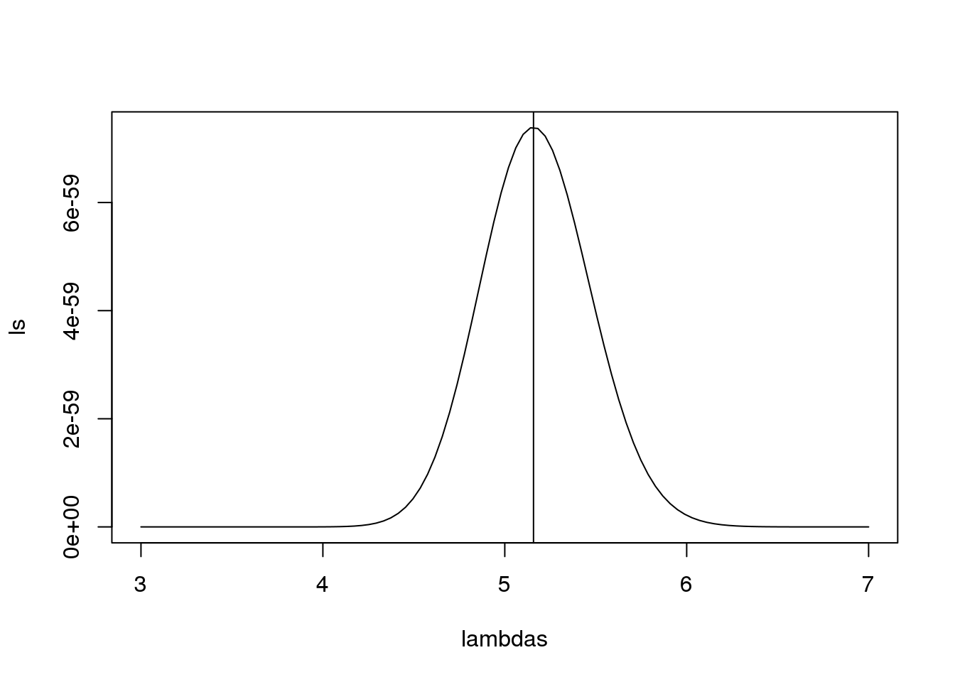

图 7.1: Likelihood versus lambda.

  通过数学运算和一点微分运算，你会意识到在这个例子中最大似然估计是其均值。

print( c(mle$maximum, mean(counts) ) )

## [1] 5.158 5.158

  需要指出的是，图中观测值和泊松分布模型的预测值一致性很高，说明泊松分布模型很适合在这个例子。

theoretical<-qpois((seq(0,99)+0.5)/100,mean(counts))

qqplot(theoretical,counts)
abline(0,1)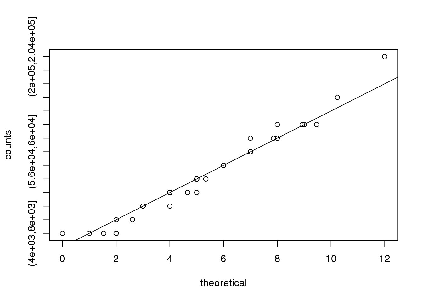

(#fig:obs_versus_theoretical_Poisson_count)Observed counts versus theoretical Poisson counts.

  因此，我们可以使用泊松分布来对回文序列的个数建模，该模型中\(\lambda=5.16\)。

7.4 连续变量的分布

在不同的生物学重复中，不同的基因差异有着不同的变化。稍后，在介绍贝叶斯层次模型的章节中，我们将介绍在基因组学数据中最具影响力的统计模型。在鉴定差异表达基因时，这种方法相对朴素的方法有着巨大的优势。这种优势是通过对方差进行建模实现的。这里我们将介绍这种方法中的参数模型。

  我们想对基因特异的标准差的分布进行建模。这种分布符合正太分布的？记住我们是在对总体的标准差进行建模，所以即使我们有成千上万个基因，中心极限定理在这里并不适用。

  我们使用一个小鼠中包含有技术重复和生物学重复的基因表达数据作为例子。我们将读入数据并计算技术重复和生物学重复中基因特异的样本标准差。

library(Biobase) ##available from Bioconductor
library(maPooling) ##available from course github repo

data(maPooling)
pd=pData(maPooling)

##determine which samples are bio reps and which are tech reps
strain=factor(as.numeric(grepl("b",rownames(pd))))
pooled=which(rowSums(pd)==12 & strain==1)
techreps=exprs(maPooling[,pooled])
individuals=which(rowSums(pd)==1 & strain==1)

##remove replicates
individuals=individuals[-grep("tr",names(individuals))]
bioreps=exprs(maPooling)[,individuals]

###now compute the gene specific standard deviations
library(matrixStats)
techsds=rowSds(techreps)
biosds=rowSds(bioreps)

  现在我们现在可以来探索一下样本的标准差：

###now plot
library(rafalib)
mypar()
shist(biosds,unit=0.1,col=1,xlim=c(0,1.5))
shist(techsds,unit=0.1,col=2,add=TRUE)
legend("topright",c("Biological","Technical"), col=c(1,2),lty=c(1,1))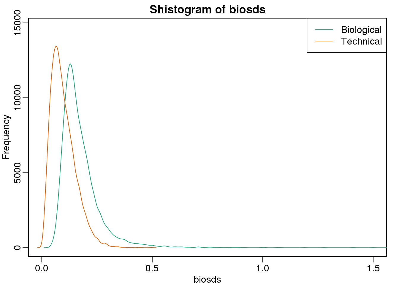

(#fig:bio_sd_versus_tech_sd)Histograms of biological variance and technical variance.

  从图中我们可以看到，生物学重复的变异显著的比技术重复之间的变异高。这表明，基因特异的生物学差异确实是存在的。

  如果我们想对这种变异建模，正态分布首先是不合适的，因为图中分布右尾相当明显。同时，因为标准差总是正数，所以其分布是无法对称的。

  QQ图可以很直观的表达这一点：

qqnorm(biosds)
qqline(biosds)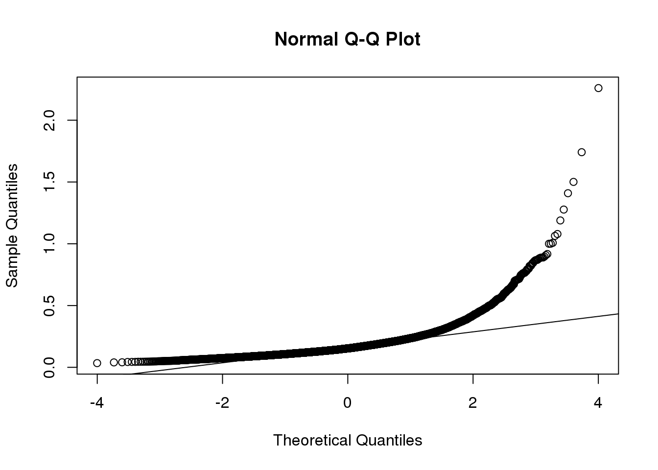

(#fig:sd_qqplot)Normal qq-plot for sample standard deviations.

  有一些参数分布可以对正数和重右尾的数据建模，例如_gamma_和_F_分布。其中_gamma_分布的密度函数是：

\[ f(x;\alpha,\beta)=\frac{\beta^\alpha x^{\alpha-1}\exp{-\beta x}}{\Gamma(\alpha)} \]

  公式中的\(\alpha\)和\(\beta\)可以间接的控制分布的位置和重尾（heavy tail）的程度，进而控制了分布的形状。如果你想了解更多关于这个分布的内容，请参考这本书.

  伽玛分布的两个特列是卡平方分布和指数分布分布。前面我们已经用到卡平方来分析一个2x2的列表数据。对于卡平方，\(\alpha=\nu/2\)，\(\beta=2\)，同时自由度为\(\nu\)。对于指数分布，\(\alpha=1\)，同时\(\beta=\lambda\)。

  F分布会在方差分析（ANOVA）中讲到。F分布，变量总是正值同时在右侧有重尾。该分布中，两个参数决定其形状：

\[ f(x,d_1,d_2)=\frac{1}{B\left( \frac{d_1}{2},\frac{d_2}{2}\right)} \left(\frac{d_1}{d_2}\right)^{\frac{d_1}{2}} x^{\frac{d_1}{2}-1}\left(1+\frac{d1}{d2}x\right)^{-\frac{d_1+d_2}{2}} \]

7.4.0.1 方差建模

  在稍后的章节中，我们会介绍通过层次模型会提高方差估计。

\[ s^2 \sim s_0^2 F_{d,d_0} \]

with \(d\) the degrees of freedom involved in computing \(s^2\). For example, in a case comparing 3 versus 3, the degrees of freedom would be 4. This leaves two free parameters to adjust to the data. Here \(d\) will control the location and \(s_0\) will control the scale. Below are some examples of \(F\) distribution plotted on top of the histogram from the sample variances:

library(rafalib)
mypar(3,3)
sds=seq(0,2,len=100)
for(d in c(1,5,10)){
  for(s0 in c(0.1, 0.2, 0.3)){
    tmp=hist(biosds,main=paste("s_0 =",s0,"d =",d),
      xlab="sd",ylab="density",freq=FALSE,nc=100,xlim=c(0,1))
    dd=df(sds^2/s0^2,11,d)
    ##multiply by normalizing constant to assure same range on plot
    k=sum(tmp$density)/sum(dd) 
    lines(sds,dd*k,type="l",col=2,lwd=2)
    }
}

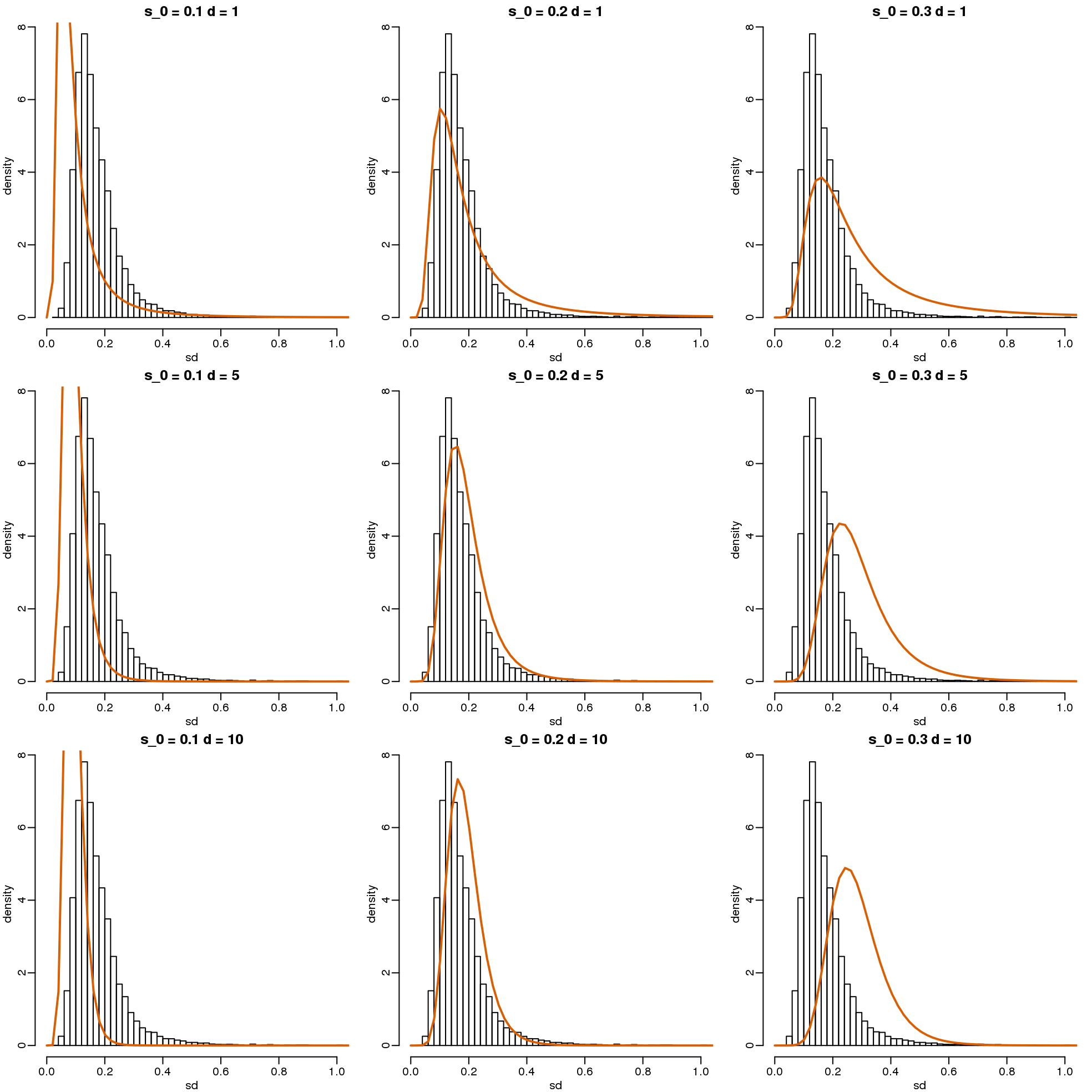
(#fig:modeling_variance)Histograms of sample standard deviations and densities of estimated distributions.

Now which \(s_0\) and \(d\) fit our data best? This is a rather advanced topic as the MLE does not perform well for this particular distribution (we refer to Smyth (2004)). The Bioconductor limma package provides a function to estimate these parameters:

library(limma)
estimates=fitFDist(biosds^2,11)

theoretical<- sqrt(qf((seq(0,999)+0.5)/1000, 11, estimates$df2)*estimates$scale)
observed <- biosds

The fitted models do appear to provide a reasonable approximation, as demonstrated by the qq-plot and histogram:

mypar(1,2)
qqplot(theoretical,observed)
abline(0,1)
tmp=hist(biosds,main=paste("s_0 =", signif(estimates[[1]],2),
                  "d =", signif(estimates[[2]],2)),
  xlab="sd", ylab="density", freq=FALSE, nc=100, xlim=c(0,1), ylim=c(0,9))
dd=df(sds^2/estimates$scale,11,estimates$df2)
k=sum(tmp$density)/sum(dd) ##a normalizing constant to assure same area in plot
lines(sds, dd*k, type="l", col=2, lwd=2)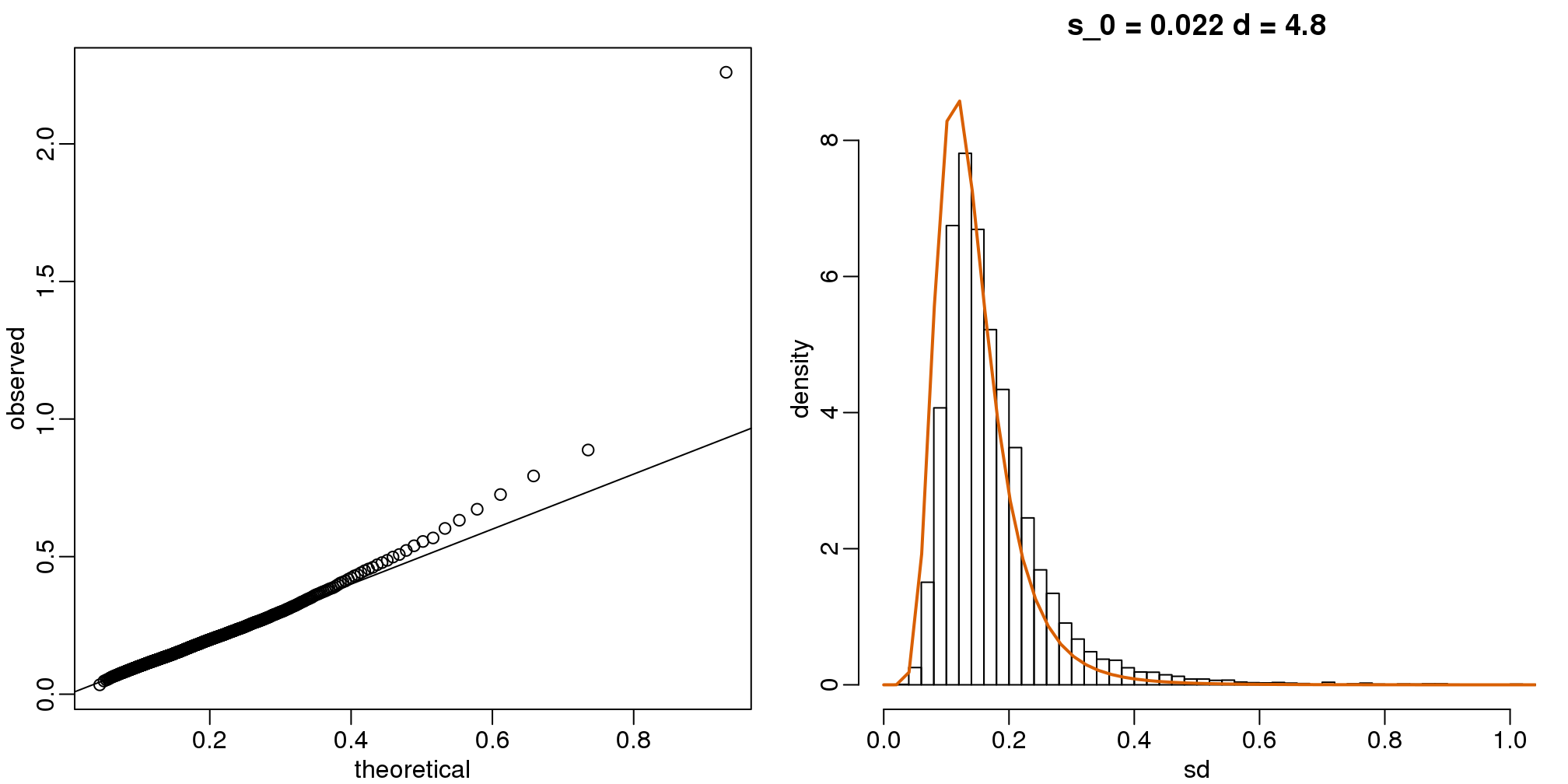

(#fig:variance_model_fit)qq-plot (left) and density (right) demonstrate that model fits data well.

7.5 贝叶斯统计

  高通量数据的一个突出特点是尽管我们想要研究一些特殊的特征值，但是通常我们也观察多许多相关的其他内容。例如，通过RNA-seq我们能够衡量成千上万个基因的表达量，利用ChIP-seq我们可以计算成千上万个峰的高度（象征蛋白结合强度），利用BS-seq我们可以计算几个CpG位点的甲基化水平。然而，前面我们介绍的大多数的统计推断方法将每一个特征值看成是独立的，因此并没有考虑其他特征值。

7.5.0.1 贝叶斯定理

  首先，我们来回顾一下贝叶斯定理。我们利用一个假设的囊性纤维化检测试验作为一个例子。假设，该测试试验的准确性是99%。我们将会有下面的公式：

\[ \mbox{Prob}(+ \mid D=1)=0.99, \mbox{Prob}(- \mid D=0)=0.99 \]

  \(+\)表示检测结果为阳性，\(D\)表示受试者实际患病（1）或者未患病（0）。

  假设我们随机选取一个人测试，该受试者测试结果为阳性，那么他患病的概率是多少？

\[ \mbox{Pr}(A \mid B) = \frac{\mbox{Pr}(B \mid A)\mbox{Pr}(A)}{\mbox{Pr}(B)} \]

  这个公式应用到我们的问题中，我们得到:

\[ \begin{align*} \mbox{Prob}(D=1 \mid +) & = \frac{ P(+ \mid D=1) \cdot P(D=1)} {\mbox{Prob}(+)} \\ & = \frac{\mbox{Prob}(+ \mid D=1)\cdot P(D=1)} {\mbox{Prob}(+ \mid D=1) \cdot P(D=1) + \mbox{Prob}(+ \mid D=0) \mbox{Prob}( D=0)} \end{align*} \]

  代入具体的数据，我们得到下面的结果:

\[ \frac{0.99 \cdot 0.00025}{0.99 \cdot 0.00025 + 0.01 \cdot (.99975)} = 0.02 \]

  这个结果表明，尽管检测准确性很高，能够达到0.99。但是在检测结果为阳性的情况下，受试者患病的概率却只有0.02。这看起来和我们的直觉是是相反的。得到这个结果的原因是在我们随机选取的这个受试者患病的概率极低。为了更直观的解释这个结果，我们使用蒙特·卡罗方法模拟一个数据。

7.5.0.2 模拟

  下面的模拟是为了帮助你更直观的理解贝叶斯定理。首先，我们从一个患病率为5%的群体中随机选取1500个人。

set.seed(3)
prev <- 1/20
##Later, we are arranging 1000 people in 80 rows and 20 columns
M <- 50 ; N <- 30
##do they have the disease?
d<-rbinom(N*M,1,p=prev)

  接着我们队每一个人进行测试，测试的准确性是99%。

accuracy <- 0.9
test <- rep(NA,N*M)
##do controls test positive?
test[d==1]  <- rbinom(sum(d==1), 1, p=accuracy)
##do cases test positive?
test[d==0]  <- rbinom(sum(d==0), 1, p=1-accuracy)

   因为对照的个数远远大于病例的个数，所以即使假阳性率比较低的情况下，我们在检测结果为阳性的这一组中依然看到对照的个数大于患病的个数（此处图对应的代码没有显示）。

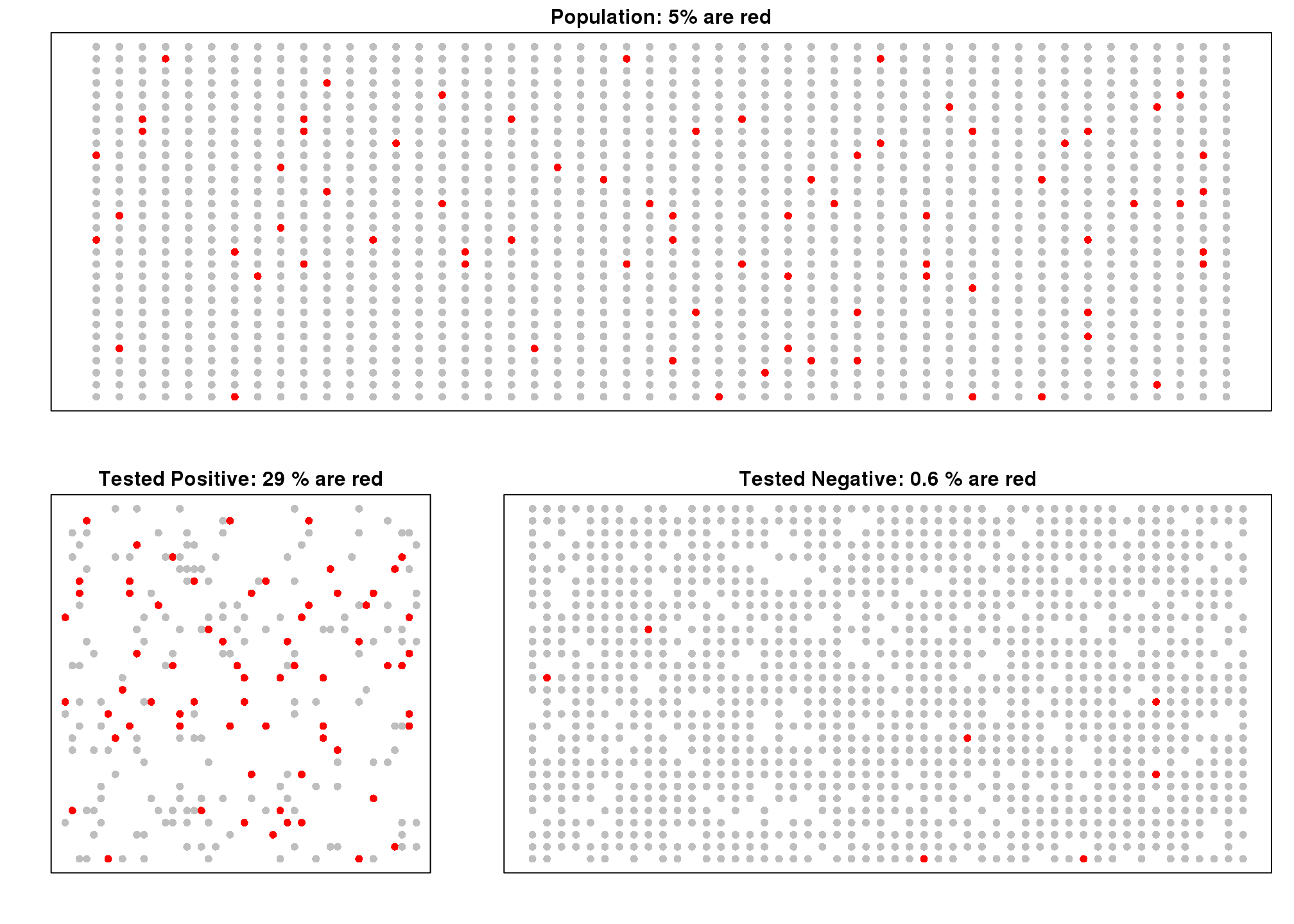
图 7.2: Simulation demonstrating Bayes theorem. Top plot shows every individual with red denoting cases. Each one takes a test and with 90% gives correct answer. Those called positive (either correctly or incorrectly) are put in the bottom left pane. Those called negative in the bottom right.

  在上图中，上半部分红色比例代表\(\mbox{Pr}(D=1)\)。左下图代表\(\mbox{Pr}(D=1 \mid +)\)。左下图代表\(\mbox{Pr}(D=0 \mid +)\)。

  José Iglesias是一个职业的棒球运动员。2013年4月是他职业生涯的第一个月，他的表现非常棒:

Month	At Bats	H	AVG
April	20	9	.450

  棒球的击球率（AVG：the batting average）是衡量一个棒球员表现的一个指标。通常来讲，AVG表示击球成功的概率。0.450的AVG是非常好的一个表现。例如，1941年传奇棒球球员Ted Williams的AVG为0.406，从那以后没有一个球员能够取得这么好的成绩。为了解释分层模型是非常有效的，我们将试着利用José的超过500次的急求数据来预测其整个赛季的AVG。

  截止现在，我们所学到的内容都属于频率学派统计学，我们能做到的是提供一个置信区间。我们讲击球事件看做一个成功率为\(p\)的二项分布。所以如果\(p\)是0.450，20次击球的标准差是：

\[ \sqrt{\frac{.450 (1-.450)}{20}}=.111 \]

  这说明我们的执行区间是0.228（.450-.222）到0.672（.450+.222）。

  这个预测有两个问题。首先，置信区间太大，所以没有实际意义。另外，该预测的中心是0.450（即我们的最佳预测），表明我们的最佳预测是这名新球员的AVG可能会打破Ted Williams在1941年创下的记录。如果你关注棒球，你会认为这个预测是有很大问题的。这是因为你已经在使用层次模型了，你将你几年来关注棒球得到的信息以一种直觉的形式来判断这一问题了。接下来我们将介绍我们如果以数学的形式来量化这种直觉。

  首先，让我们先来看看在前三个赛季中击球数超过500次的球员的平均AVG：

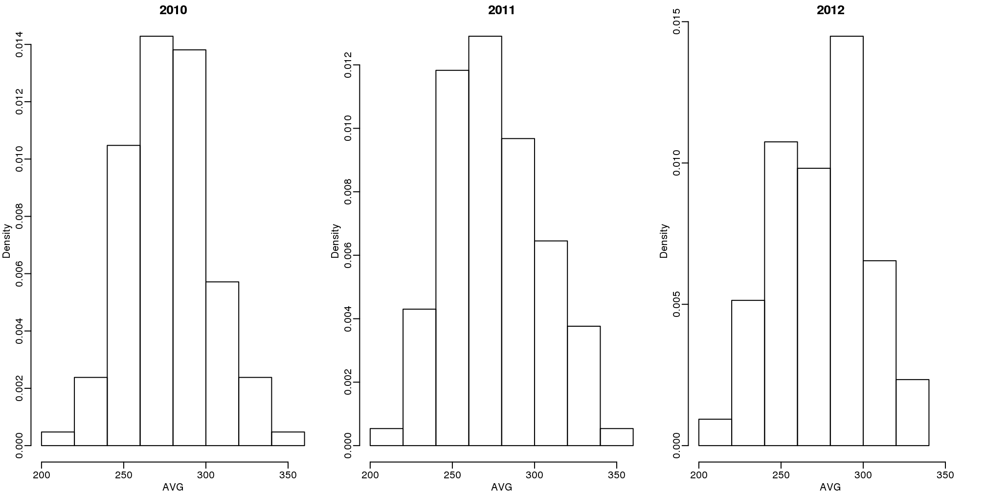
(#fig:batting_averages)Batting average histograms for 2010, 2011, and 2012.

  我们会发现，棒球球员的AVG均值是0.275，标准差是0.027。所以我们已经可以看出0.450的AVG是非常异常的，这个值偏离均值超过6个标准差。所以José有0.450这个成绩是碰巧的还是说他确实是自1941年以来最好的球员呢？这可能两者的因素都有。但是碰巧的因素和他确实有这么好的概率有多少呢?这样的判断会对球员交易产生影响。如果，经过分析我们认为他只是碰巧取得了这个成绩，他并没有那么好，那么你作为球队老板可能就会选择将他交易到其他球队，也许其他球队会根据0.450这个数据尔高估他，认为他确实非常优秀。

7.5.0.3 层次模型

  层次模型提供了一种让方法让我们能够用数学的语言来描述这一例子。首先，我们随机选取了一个优秀的球员，这个选择是基于\(\theta\)。\(\theta\)是根据20次随机事件得出的一个成功概率。

\[ \begin{align*} \theta &\sim N(\mu, \tau^2) \mbox{ describes randomness in picking a player}\\ Y \mid \theta &\sim N(\theta, \sigma^2) \mbox{ describes randomness in the performance of this particular player} \end{align*} \]

```   这里有两个层次的意思：1）球员和球员之间的差异；2）击球时运气因素引起的变异。在贝叶斯模型中，第一层次称之为_先验概率_，第二层次为_样本分布_。

  现在，让我们用层次模型来对José的数据进行建模。假设我们的目的是预测他__真实__的击球率来评估他的天赋。下面展示的是这一数据的层次模型：

\[ \begin{align*} \theta &\sim N(.275, .027^2) \\ Y \mid \theta &\sim N(\theta, .111^2) \end{align*} \]

  现在我们可以计算后验概率分布来预测\(\theta\)。贝叶斯法则的连续版本可以被用来推断_后验概率_，这也是从观测数据中的参数 \(\theta\)的缝补。

\[ \begin{align*} f_{ \theta \mid Y} (\theta\mid Y) &= \frac{f_{Y\mid \theta}(Y\mid \theta) f_{\theta}(\theta) }{f_Y(Y)}\\ &= \frac{f_{Y\mid \theta}(Y\mid \theta) f_{\theta}(\theta)} {\int_{\theta}f_{Y\mid \theta}(Y\mid \theta)f_{\theta}(\theta)} \end{align*} \]

  我们尤其对能够使后验概率\(f_{\theta\mid Y}(\theta\mid Y)\)取得最大值的\(\theta\)。在我们的数据中，我们可以看到后验概率的分布符合正态分布，我们也可以计算均值\(\mbox{E}(\theta\mid y)\)和方差\(\mbox{var}(\theta\mid y)\)。我们可以具体一下面的形式展示该分布的均值。

\[ \begin{align*} \mbox{E}(\theta\mid y) &= B \mu + (1-B) Y\\ &= \mu + (1-B)(Y-\mu)\\ B &= \frac{\sigma^2}{\sigma^2+\tau^2} \end{align*} \]

It is a weighted average of the population average \(\mu\) and the observed data \(Y\). The weight depends on the SD of the population \(\tau\) and the SD of our observed data \(\sigma\). This weighted average is sometimes referred to as shrinking because it shrinks estimates towards a prior mean. In the case of José Iglesias, we have:

\[ \begin{align*} \mbox{E}(\theta \mid Y=.450) &= B \times .275 + (1 - B) \times .450 \\ &= .275 + (1 - B)(.450 - .275) \\ B &=\frac{.111^2}{.111^2 + .027^2} = 0.944\\ \mbox{E}(\theta \mid Y=450) &\approx .285 \end{align*} \]

The variance can be shown to be:

\[ \mbox{var}(\theta\mid y) = \frac{1}{1/\sigma^2+1/\tau^2} = \frac{1}{1/.111^2 + 1/.027^2} = 0.00069 \] and the standard deviation is therefore \(0.026\). So we started with a frequentist 95% confidence interval that ignored data from other players and summarized just José’s data: .450 \(\pm\) 0.220. Then we used a Bayesian approach that incorporated data from other players and other years to obtain a posterior probability. This is actually referred to as an empirical Bayes approach because we used data to construct the prior. From the posterior we can report what is called a 95% credible interval by reporting a region, centered at the mean, with a 95% chance of occurring. In our case, this turns out to be: .285 \(\pm\) 0.052.

The Bayesian credible interval suggests that if another team is impressed by the .450 observation, we should consider trading José as we are predicting he will be just slightly above average. Interestingly, the Red Sox traded José to the Detroit Tigers in July. Here are the José Iglesias batting averages for the next five months.

Month	At Bat	Hits	AVG
April	20	9	.450
May	26	11	.423
June	86	34	.395
July	83	17	.205
August	85	25	.294
September	50	10	.200
Total w/o April	330	97	.293

Although both intervals included the final batting average, the Bayesian credible interval provided a much more precise prediction. In particular, it predicted that he would not be as good the remainder of the season.

7.6 Hierarchical Models

In this section, we use the mathematical theory which describes an approach that has become widely applied in the analysis of high-throughput data. The general idea is to build a hierachichal model with two levels. One level describes variability across samples/units, and the other describes variability across features. This is similar to the baseball example in which the first level described variability across players and the second described the randomness for the success of one player. The first level of variation is accounted for by all the models and approaches we have described here, for example the model that leads to the t-test. The second level provides power by permitting us to “borrow” information from all features to inform the inference performed on each one.

Here we describe one specific case that is currently the most widely used approach to inference with gene expression data. It is the model implemented by the limma Bioconductor package. This idea has been adapted to develop methods for other data types such as RNAseq by, for example, edgeR and DESeq2. This package provides an alternative to the t-test that greatly improves power by modeling the variance. While in the baseball example we modeled averages, here we model variances. Modelling variances requires more advanced math, but the concepts are practically the same. We motivate and demonstrate the approach with an example.

Here is a volcano showing effect sizes and p-value from applying a t-test to data from an experiment running six replicated samples with 16 genes artificially made to be different in two groups of three samples each. These 16 genes are the only genes for which the alternative hypothesis is true. In the plot they are shown in blue.

library(SpikeInSubset) ##Available from Bioconductor
data(rma95)
library(genefilter)
fac <- factor(rep(1:2,each=3))
tt <- rowttests(exprs(rma95),fac)
smallp <- with(tt, p.value < .01)
spike <- rownames(rma95) %in% colnames(pData(rma95))
cols <- ifelse(spike,"dodgerblue",ifelse(smallp,"red","black"))

with(tt, plot(-dm, -log10(p.value), cex=.8, pch=16,
     xlim=c(-1,1), ylim=c(0,4.5),
     xlab="difference in means",
     col=cols))
abline(h=2,v=c(-.2,.2), lty=2)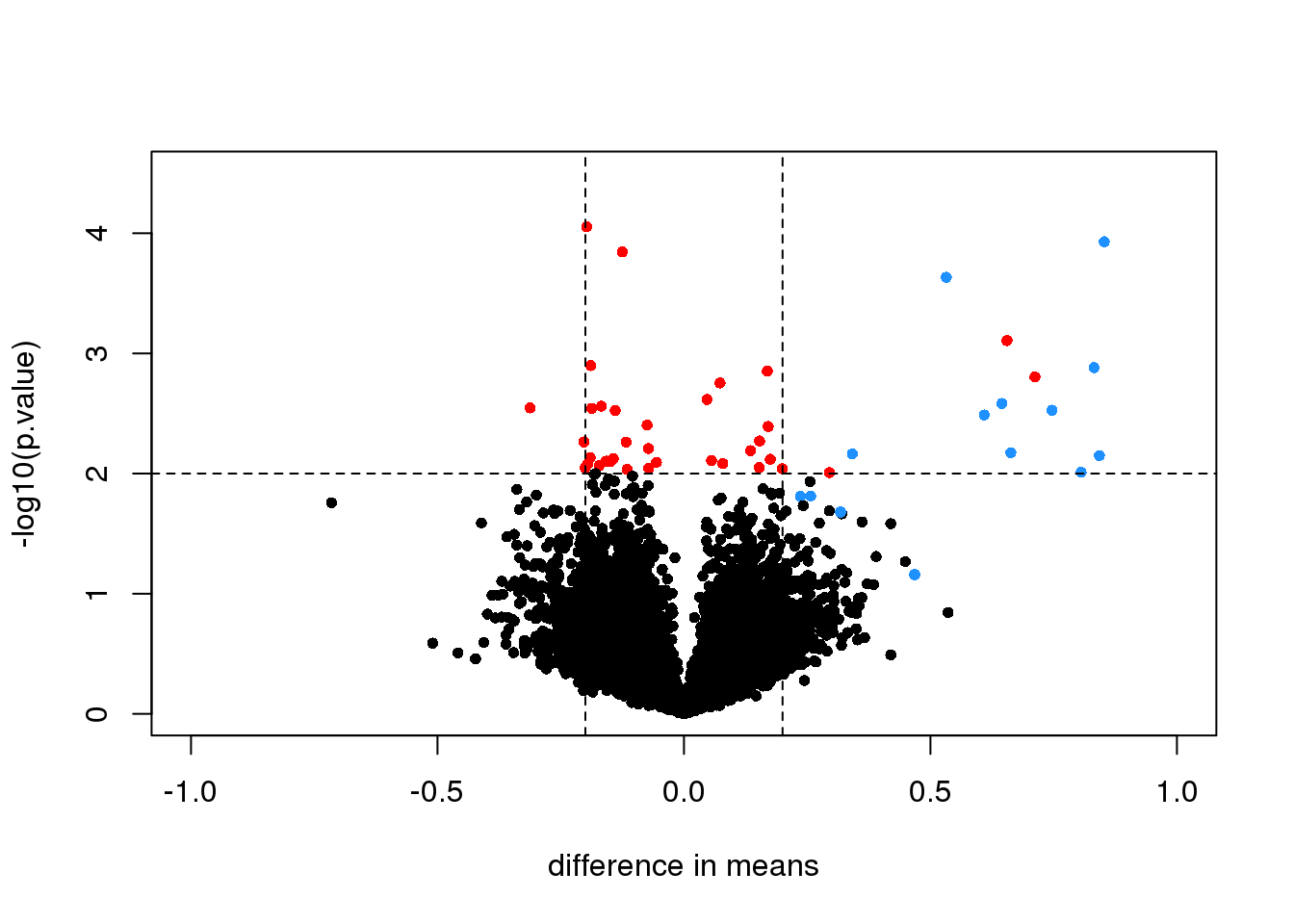

图 7.3: Volcano plot for t-test comparing two groups. Spiked-in genes are denoted with blue. Among the rest of the genes, those with p-value < 0.01 are denoted with red.

We cut-off the range of the y-axis at 4.5, but there is one blue point with a p-value smaller than \(10^{-6}\). Two findings stand out from this plot. The first is that only one of the positives would be found to be significant with a standard 5% FDR cutoff:

sum( p.adjust(tt$p.value,method = "BH")[spike] < 0.05)

## [1] 1

This of course has to do with the low power associated with a sample size of three in each group. The second finding is that if we forget about inference and simply rank the genes based on the size of the t-statistic, we obtain many false positives in any rank list of size larger than 1. For example, six of the top 10 genes ranked by t-statistic are false positives.

table( top50=rank(tt$p.value)<= 10, spike) #t-stat and p-val rank is the same

##        spike
## top50   FALSE  TRUE
##   FALSE 12604    12
##   TRUE      6     4

In the plot we notice that these are mostly genes for which the effect size is relatively small, implying that the estimated standard error is small. We can confirm this with a plot:

tt$s <- apply(exprs(rma95), 1, function(row) 
  sqrt(.5 * (var(row[1:3]) + var(row[4:6]) ) ) )
with(tt, plot(s, -log10(p.value), cex=.8, pch=16,
              log="x",xlab="estimate of standard deviation",
              col=cols))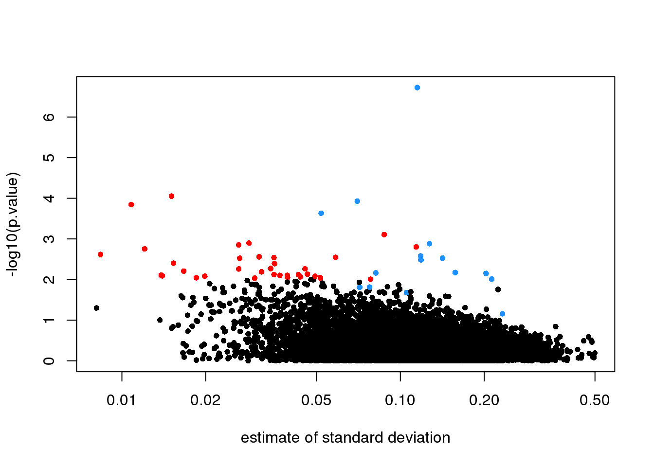

(#fig:pval_versus_sd)p-values versus standard deviation estimates.

Here is where a hierarchical model can be useful. If we can make an assumption about the distribution of these variances across genes, then we can improve estimates by “adjusting” estimates that are “too small” according to this distribution. In a previous section we described how the F-distribution approximates the distribution of the observed variances.

\[ s^2 \sim s_0^2 F_{d,d_0} \]

Because we have thousands of data points, we can actually check this assumption and also estimate the parameters \(s_0\) and \(d_0\). This particular approach is referred to as empirical Bayes because it can be described as using data (empirical) to build the prior distribution (Bayesian approach).

Now we apply what we learned with the baseball example to the standard error estimates. As before we have an observed value for each gene \(s_g\), a sampling distribution as a prior distribution. We can therefore compute a posterior distribution for the variance \(\sigma^2_g\) and obtain the posterior mean. You can see the details of the derivation in this paper.

\[ \mbox{E}[\sigma^2_g \mid s_g] = \frac{d_0 s_0^2 + d s^2_g}{d_0 + d} \]

As in the baseball example, the posterior mean shrinks the observed variance \(s_g^2\) towards the global variance \(s_0^2\) and the weights depend on the sample size through the degrees of freedom \(d\) and, in this case, the shape of the prior distribution through \(d_0\).

In the plot above we can see how the variance estimates shrink for 40 genes (code not shown):

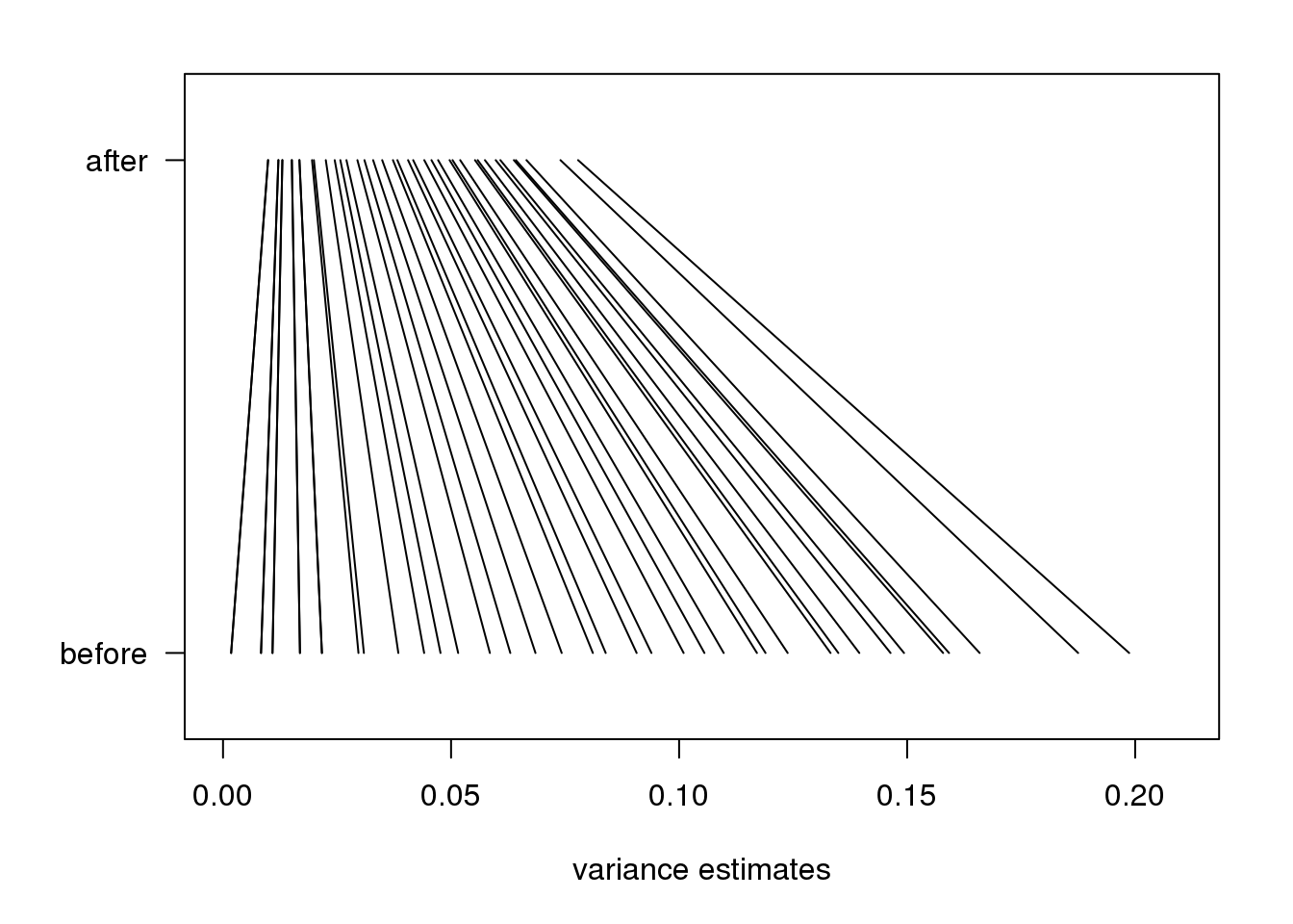
图 7.4: Illustration of how estimates shrink towards the prior expectation. Forty genes spanning the range of values were selected.

An important aspect of this adjustment is that genes having a sample standard deviation close to 0 are no longer close to 0 (they shrink towards \(s_0\)). We can now create a version of the t-test that instead of the sample standard deviation uses this posterior mean or “shrunken” estimate of the variance. We refer to these as moderated t-tests. Once we do this, the improvements can be seen clearly in the volcano plot:

library(limma)
fit <- lmFit(rma95, model.matrix(~ fac))
ebfit <- ebayes(fit)
limmares <- data.frame(dm=coef(fit)[,"fac2"], p.value=ebfit$p.value[,"fac2"])
with(limmares, plot(dm, -log10(p.value),cex=.8, pch=16,
     col=cols,xlab="difference in means",
     xlim=c(-1,1), ylim=c(0,5)))
abline(h=2,v=c(-.2,.2), lty=2)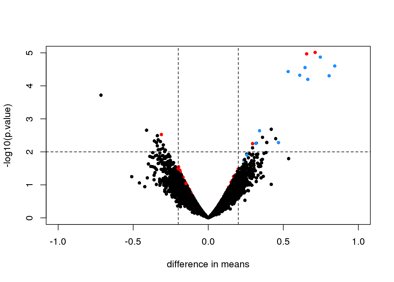

图 7.5: Volcano plot for moderated t-test comparing two groups. Spiked-in genes are denoted with blue. Among the rest of the genes, those with p-value < 0.01 are denoted with red.

The number of false positives in the top 10 is now reduced to 2.

table( top50=rank(limmares$p.value)<= 10, spike) 

##        spike
## top50   FALSE  TRUE
##   FALSE 12608     8
##   TRUE      2     8